
In the first post of our series we focused on structural dynamics and earthquake engineering. We shared examples of how our Shake Table systems are used in teaching and research labs around the world. In this post, let’s look closer on one of the most popular and well-known areas where these systems are used: earthquake engineering.
Simulating earthquakes
Besides using the Shake Tables for structural dynamics to identify, for instance, the natural frequency and damping of a structure, one of the more common application is simulating earthquakes. That is, replaying an earthquake that already occurred on the table.
There are various earthquake databases used worldwide. One example is the PEER Strong Motion Database. It is hosted by the Pacific Earthquake Engineering Research Center (PEER) headquartered at the University of California, Berkeley. Users can download displacement, velocity, and acceleration data of earthquakes recorded worldwide. The thing is, many of the earthquakes have large displacements. To simulate them on a shake table with a limited stroke, the recorded data has to be scaled down.
Q-Scale algorithm for Shake Tables
To scale down the displacement of a recorded earthquake, Quanser engineers developed a “Q-Scale” algorithm. This algorithm scales down the position and the time scale of the earthquake records but maintains the accelerations of the original earthquake. In other words, based on the earthquake acceleration record, Q-Scale computes the position that the shake table must track in order to obtain the same accelerations while keeping it below the maximum position specified. Thus users can run earthquakes on a bench-top shake table with the same accelerations as the original earthquake.
The Quanser Q-Scale algorithm was further improved in 2005 with the help of Dr. Eduardo Kausel from the Massachusetts Institute of Technology. Dr. Kausel modified the script and applied his own “baseline correction” method that adjusts the accelerations recorded from an instrument, e.g., an accelerometer, to obtain more representative accelerations.
As discussed by Dr. Kausel, “many accelerometers behave as damped one degree-of-freedom (1 DOF) systems where the frequency-response or transfer function is not flat in the frequency range of interest, nor is the phase angle linear with frequency.” Further, accelerometers often have their own analog filters to avoid aliasing, and those introduce more dynamics that prevent having an accurate 1:1 displacement record. As a result, published earthquake records are commonly corrected to compensate for that.
However, earthquake correcting methods can introduce other issues. For example, direct integration causes drift where you may not get a final displacement and velocity of zero. Having a non-zero final velocity is problematic because it indicates the ground is still moving when it is, in fact, no longer in motion.
Dr. Kausel’s baseline method
The baseline method Dr. Kausel implemented solves this to obtain an accurate ground trajectory. Using a cubic parabola data fitting equation
![]() where the variable t is the initial time. The new corrected acceleration record is
where the variable t is the initial time. The new corrected acceleration record is ![]()
The a, b, and c parameters in the cubic data fitting equation above are solved using the following criteria:
a) Zero initial and final velocity
b) Zero initial and final displacement
c) Assume the integral of squared velocity is minimal
When you run the Q-Scale algorithm, it takes the raw earthquake acceleration record, finds the corrected acceleration records, and generates the scaled displacement based on the maximum imposed displacement. The trajectory computed by Q-Scale is then used as the position command to the shake table.
Scaling the Northridge Earthquake
The Northridge Earthquake occurred in California on Jan 17, 1994. We download the acceleration record from the PEER Ground Motion Database.
At a certain measurement station, the peak acceleration and displacement of Northridge reached 0.60 g and 16.9 cm. The trajectory recorded at that station is shown in the two left plots in the figure below as ‘Earthquake Acceleration (g)’ and ‘Earthquake Position (cm).’ Because the stroke of the Shake Table II is ±7.5 cm (physical limit, the effective operating range is less), this record to be scaled down. When processed by the Q-Scale algorithm, the acceleration amplitude is maintained (notice the peak acceleration is kept at 0.60 g) and the displacement is scaled-down to a pre-defined maximum position of ±3 cm (you can change this). The position and acceleration records from the Q-Scale algorithm are shown on the right side in the figure as Table Acceleration (g) and Table Position (cm) plots.
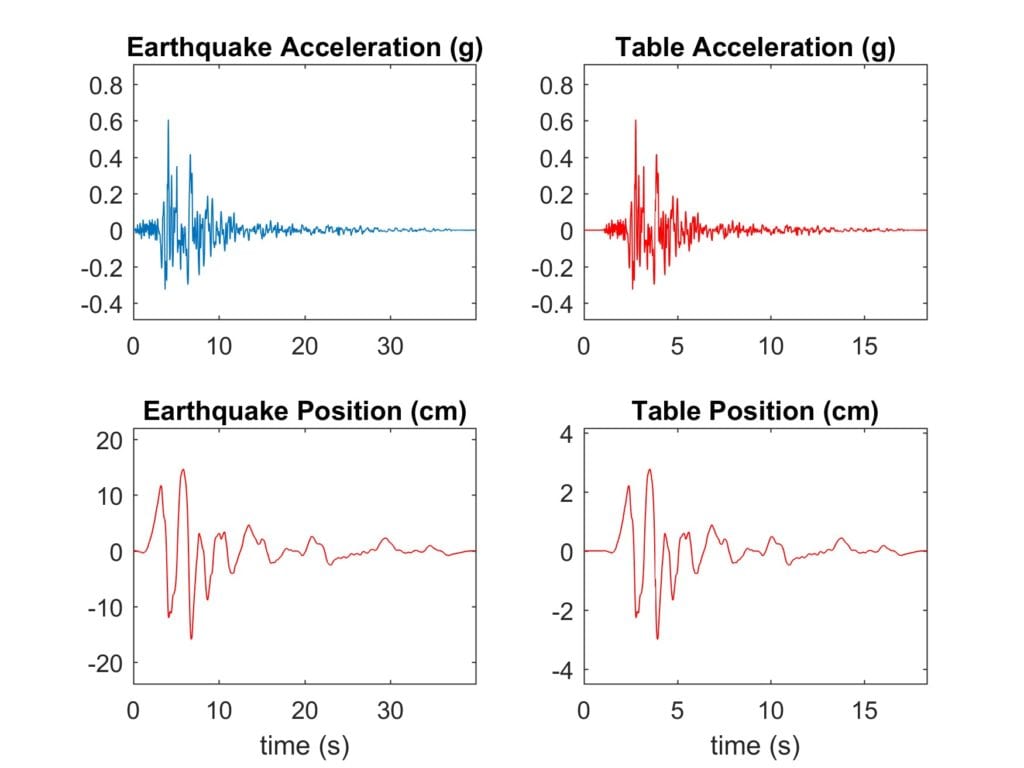
Looking at the scaling statistics gives the following information:
Original time step:    0.02000
Step 1 of 3: Get displacements
Step 2 of 3: Scale records
Ratio of table displacement to ground displacement: 0.188454

Step 3 of 3: Scaling time
Time step after scaling = 0.008682
*** Done ***
   Displacement scaled from original movement of 15.92 cm to 3.00 cm
   Time scaled from original duration of 39.98 s to 17.36 s
   Record size  =  2115 samples
Notice that to keep the same acceleration, the duration of the tremor is shrunk down from 39.98 sec down to 17.36 sec.
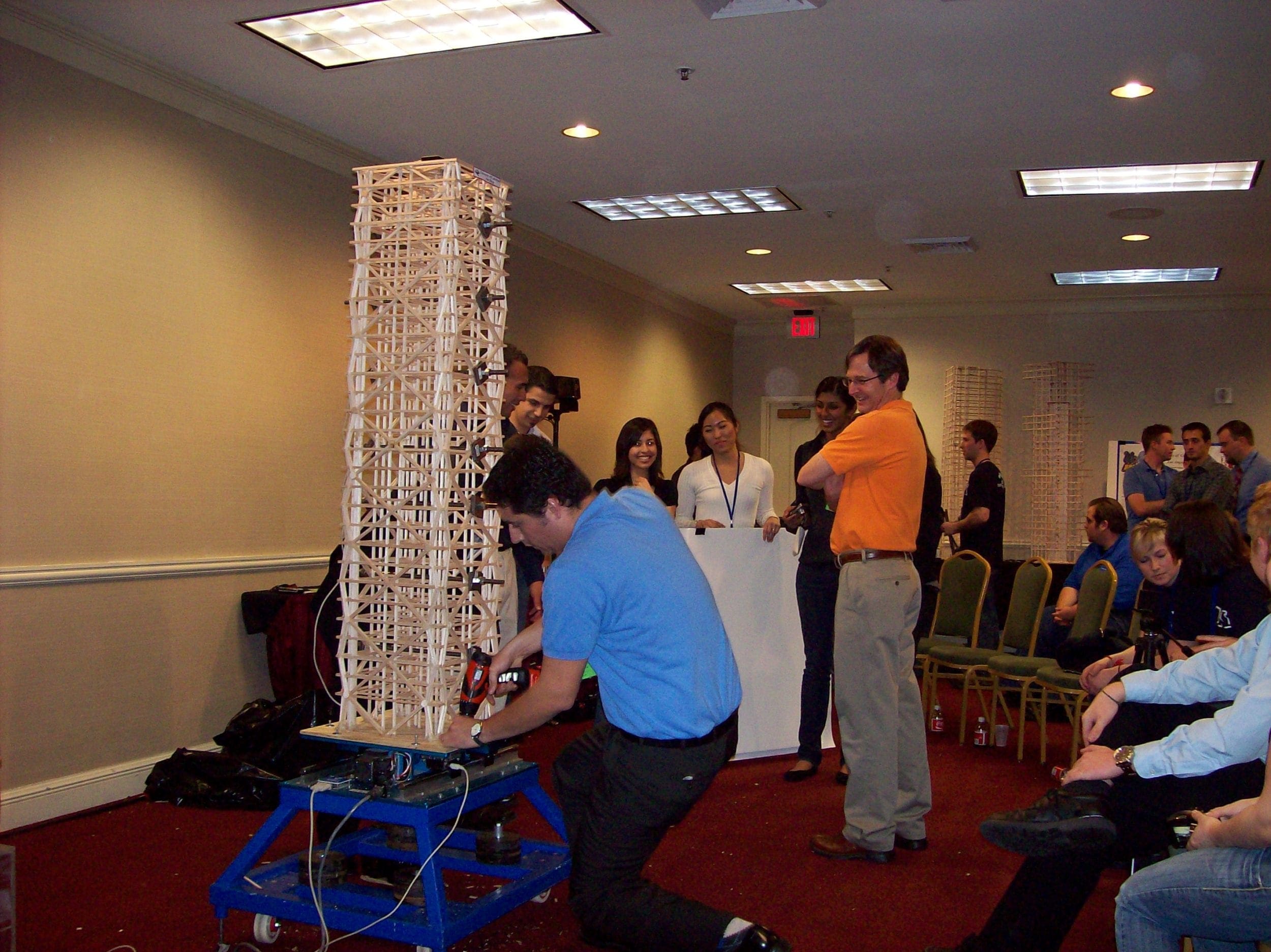
Real-life earthquake in the lab
Using ground motions from actual earthquakes makes the lab more interesting. Motivation is key, and students would rather see their building stand up to the Northridge, or some other earthquake than a pre-defined sinusoidal. See how much fun students have with testing their structures at the Annual EERI Undergraduate Student Design Competition: