
Ever since we released our Self-Driving Car Research Studio (SDRS), I’ve dedicated some of my time to finding innovative ways to push the boundaries of what’s possible and exciting with our offering. In this blog I am going to talk about how I utilized the MATLAB Navigation Toolbox to establish a global frame and localize two autonomous vehicles, as well as use our QUARC™ Communication blockset to enable intercommunication between them.
H is for Hockey
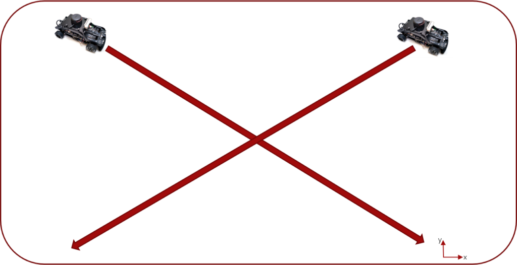
If you are a hockey fan like me, the diagram below will be familiar to you. Yes, it’s an outline of a hockey rink! Since working remotely from home, I’ve taken over my children’s basement hockey rink, doubling it as a research studio. It’s a great space to highlight some of the capabilities of the SDRS.
The Challenge ….
A couple of weeks ago I decided to challenge myself to develop a set of algorithms that would (a) generate a fixed global frame and localize two vehicles in the same map, (b) command two vehicles to drive to various locations, and (c) allow the vehicles to share data with one another.
So hopefully as I describe the experience below, you’ll get a glimpse of some of the capabilities and some of the options you will have as a researcher in this exciting field.
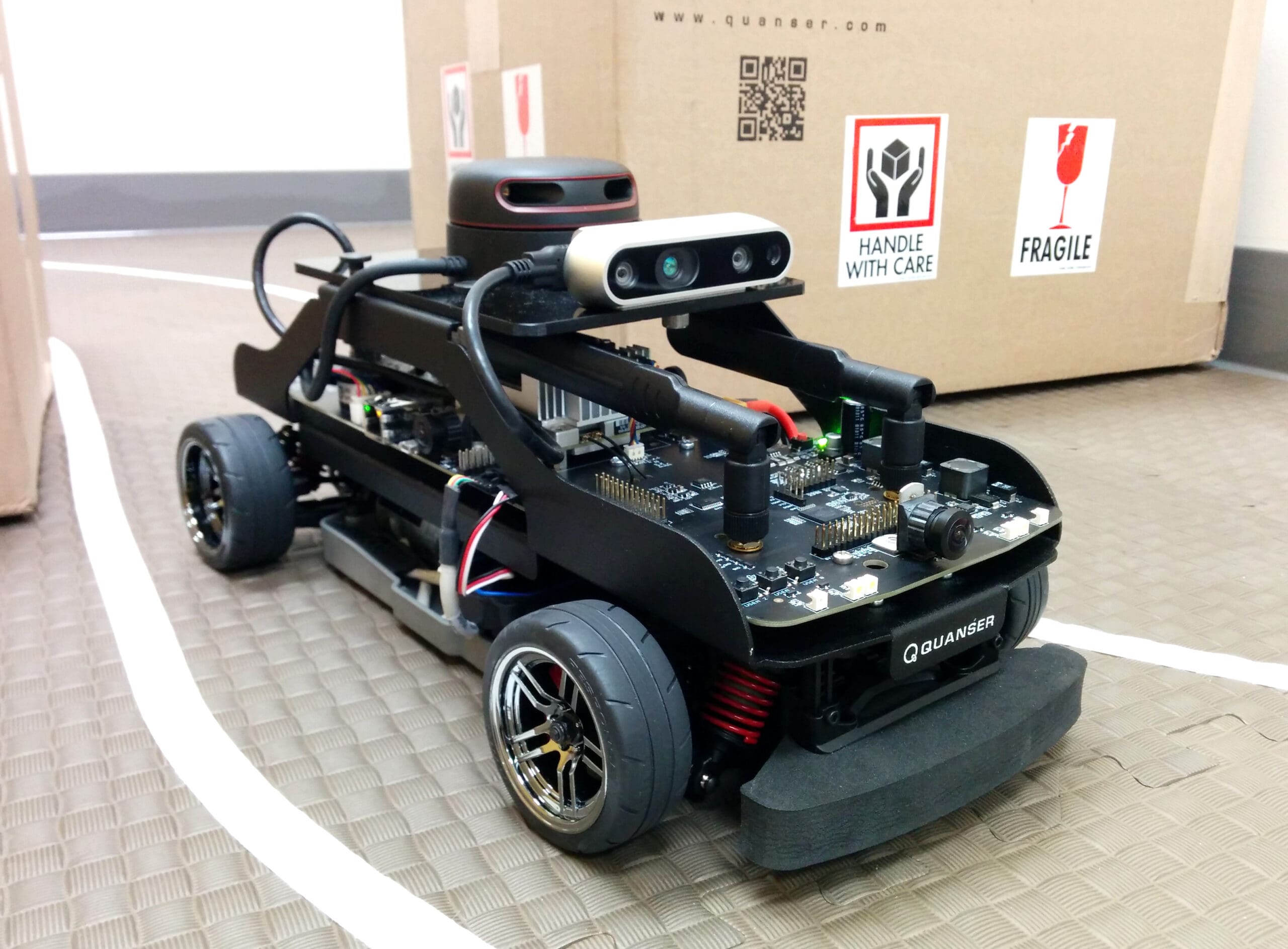
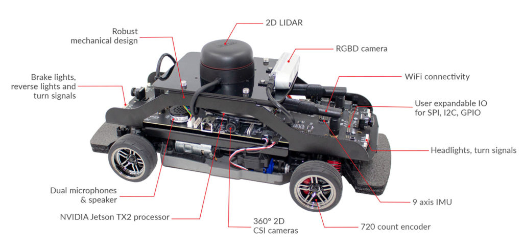
I started my exploration with two Quanser QCars, which are high-fidelity mobile computing platforms on four wheels with many sensors that are relevant to the self-driving cars applications. When we started development of this platform a few years ago, one of the key design choices was to support not just the MATLAB/Simulink environment that we typically do for many of our systems, but to also give users the versatility to use other environments that have progressed quite well in this space such as Python, ROS, TensorFlow. For my application, I was hoping to rely on ROS’s Hector SLAM algorithm to provide me some self-localization functionality. That is, depending on where I start and as I move around a given space, the algorithm will keep track of my relative position from the starting point. I then planned to run the same algorithm on both cars and my initial hypothesis was that if I started both at known locations, with those coordinates I’d then be able to extract a global reference frame for both cars to operate in. Finally, I was going to publish the ROS information to a MATLAB or Simulink model, do some addition sensor fusion, and eventually have that information communicated between the cars.
Unfortunately, as I was developing this and leveraging the Hector SLAM algorithm, being a Simulink user, I wasn’t comfortable going down to the ROS level and debugging my algorithm. I’m sure if I was back in the office and had my full team’s support, I would have been able to successfully tackle the ROS side.
Knowing that these tools did exist in the MATLAB/Simulink environment, I put aside ROS and decided to try the MATLAB Navigation Toolbox. While many MATLAB tools are for post- or offline-processing, I wanted to see if I can leverage them in real-time to achieve my objective of globally localizing both vehicles. In hindsight it was probably a little ambitious as I put in some late-night hours, but at the end of it, it was all worthwhile and forced me to learn a lot and I was able to highlight some of the interesting capabilities over and above what we currently provide in our self-driving car research studio.
At the heart of the QCar is the NVIDIA® Jetson™ TX2 processor. They stand out as being leaders of the pack because they provide fantastic processing capabilities, and they couple that with their GPU technology. Together it enables you to push the boundaries of research with the QCar. We also over instrumented the QCar by providing four cameras that you can stitch together to get full 360 view, as well as a forward-facing Intel RealSense RGBD and depth camera. But in my application, I used the QCar’s 2D lidar. Like many, I had some knowledge about lidar technology, but after what I experienced over several weeks, I developed a deeper appreciation of the capabilities.
As I started exploring the Navigation Toolbox, I quickly realized the existence of a wealth of built-in examples. It allowed me to quickly get a simple application up and running. The video below shows the post-processed results of my first test as the car autonomously drove around my basement (you can see the hockey net on the right). Each time the lidar did a scan it would fuse it and come up with a refined pose estimate. This worked very well offline. But as I attempted to do this in real-time, the data quickly became overwhelming and my PC wasn’t able to keep up with the multitudes of scans that the lidar was generating. It seemed that it wasn’t configured to be implemented in real-time as the vehicle drove around. So, I was a little concerned at this point telling myself that maybe trying to achieve a global frame in real-time is going to be harder than I thought.
Eureka!
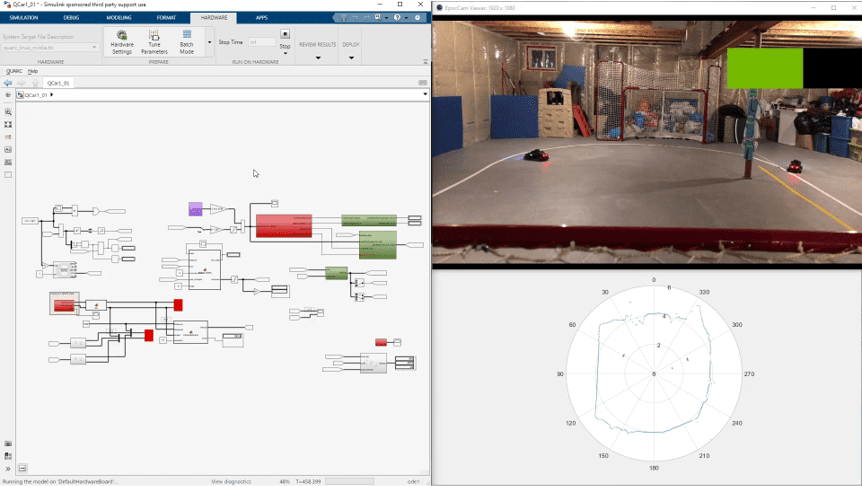
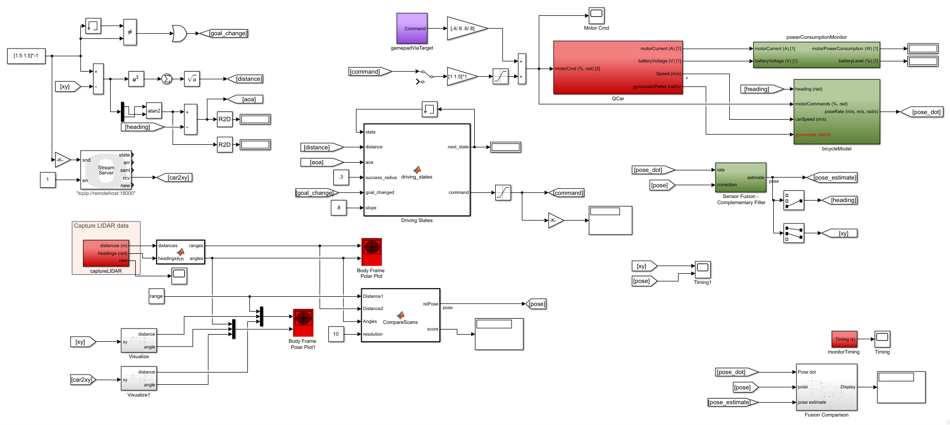
With a bit more digging I came across a paper published by Hess et al. [1], which was referenced in the toolbox documentation. They had developed an algorithm which is called matchScansGrid() in the Navigation Toolbox. The function takes two relative lidar scans and tries to give a pose estimate of one relative to the other – essentially what my goal was. An added benefit was that the algorithm was code generation compatible, meaning I could implement it in my Simulink diagram and generate optimized real-time C code for it. Using this function, I put together the model shown below. I’ll go through its main components in a moment.
Below is one of my first success videos using the model above on a single car. The map shown is generated from the first lidar scan, which I use as my global frame. As the car drives around, progressive lidar scans are compared to my global frame scan and the position and orientation of the vehicle are estimated and plotted in the graph (the blue blob moving around is the car). As you can see, it does a pretty good job to localize the car in the global frame.
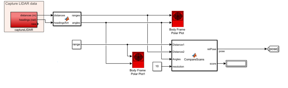
Let’s take a close look at the key components of my model. The section shown below captures the initial and subsequent lidar scans. The CompareScans embedded MATLAB function uses the matchScansGrid() function described above to compare the initial scan (Distance1) with the each progressive lidar scan (Distance2) and computes the relative pose of the vehicle with a 10 cm resolution.
But there was a small problem. Even though my lidar was scanning at 20 Hz, my algorithm was only able to extract real-time pose data at around 4 Hz, which considering the speeds at which it drives, that was not enough to localize my system. So, I had to fuse that data with something else.
Luckily, my team provided me with what we call the bicycle model of the QCar (shown below). It fuses the actual car speed (measured using the car’s onboard high-resolution encoder), yaw data (using the onboard IMU), as well as the physical parameters of the car to give me what I call pose_dot, which is an estimate of how fast my car is going. I then used a complementary filter to fuse this pose estimate (which, by the way, is computed quite fast at a rate of 1,000 Hz because it’s based on the internal sensors of the car), with the slower real pose data as my correction term (which was computed at around 4 Hz) to get my final pose estimate.
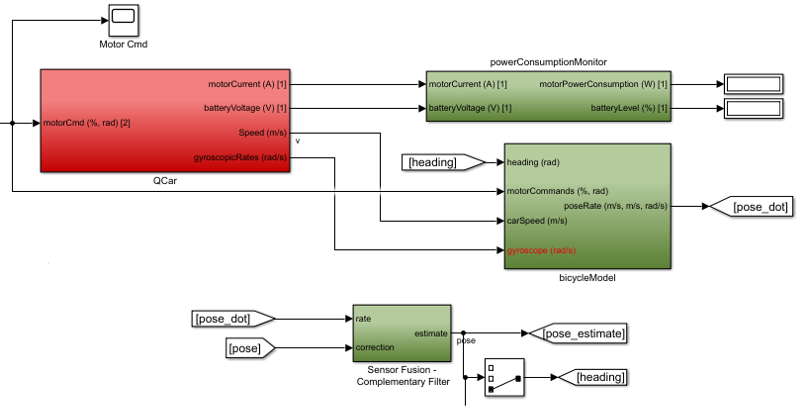
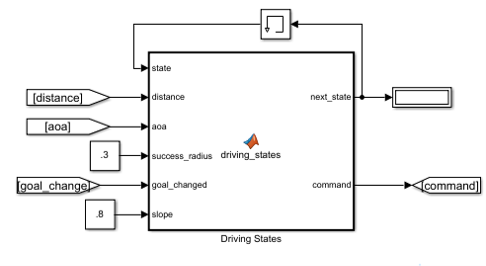
My model also implemented a simple state machine called driving_states. It has two states: (1) car has achieved the desired goal, or (2) cars driving toward the desired goal. The state machine helps minimize jitter and indecisiveness once the vehicle reached its target goal for a given success radius.
Throw in a Second Car
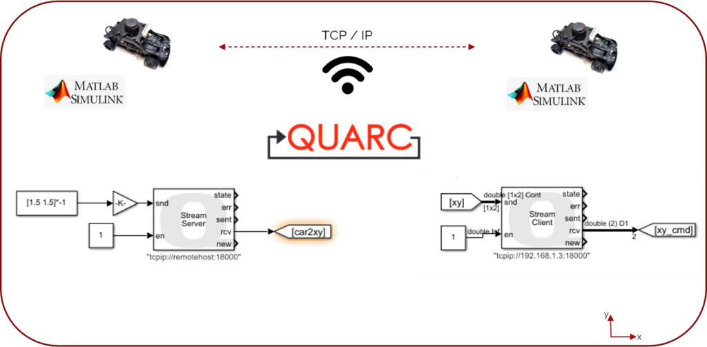
With my application working with a single vehicle, my next goal was to add in a second car and have both communicate with each other. Since I had a fixed reference from my first car, I deployed the same model to the second car. I then used our QUARC stream blocks (schematically shown below), with a Stream Server block running on the first car and a Stream Client block running on the second car. Using the TCP/IP protocol, the server sends XY destination commands over to the second car and receives back the position of the second car. While the client sends its position over to the first car and receives destination commands from the first car.
Here’s a video of my first attempt at running my model on both cars. As the models run, both cars autonomously drive off to two different commanded destinations. As you can see, even though both cars are aware of each other’s position, halfway through they collided, and that was because I had not implemented any collision avoidance.
Finally, as you can see in the video below, after a bit of tuning my model I was able to get the two cars to navigate to two different locations without colliding.
Keep in mind that the QCar is an open-architecture platform and will only take actions that they’ve been programmed with. This is a key feature that researchers appreciate about our system. For example, you can develop a centralized system that changes the motion planning based on the real-time position of each car. Or you can develop obstacle avoidance algorithms on the vehicles. All of these can be implemented because the cars share position data as well as having a multitude of sensors imbedded in the cars.
So, in summary, thanks to the Navigation Toolbox, I was able to reach my goal which was to establish a global reference frame for two cars, have two cars communicate with each other, and also command the vehicles to go to different locations inside my test area.
Hope you will find my experience useful. What MATLAB toolboxes do you use in your autonomous vehicle research? Let me know in the comments below!