
Model Predictive Control (MPC) has gained a lot of popularity over the last 15 years and for a good reason – it works well with relatively little design effort. MPC was originally developed for the process control industry. So it only made sense to test this on the Quanser Coupled Tanks using the MathWorks® Model Predictive Control Toolbox for Simulink®. In this blog MPC is implemented both on the QLabs Virtual Coupled Tanks system as well as the Quanser Coupled Tanks hardware using the QUARC Real-Time Control software.
Why use MPC for the Coupled Tanks?
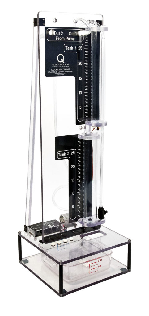
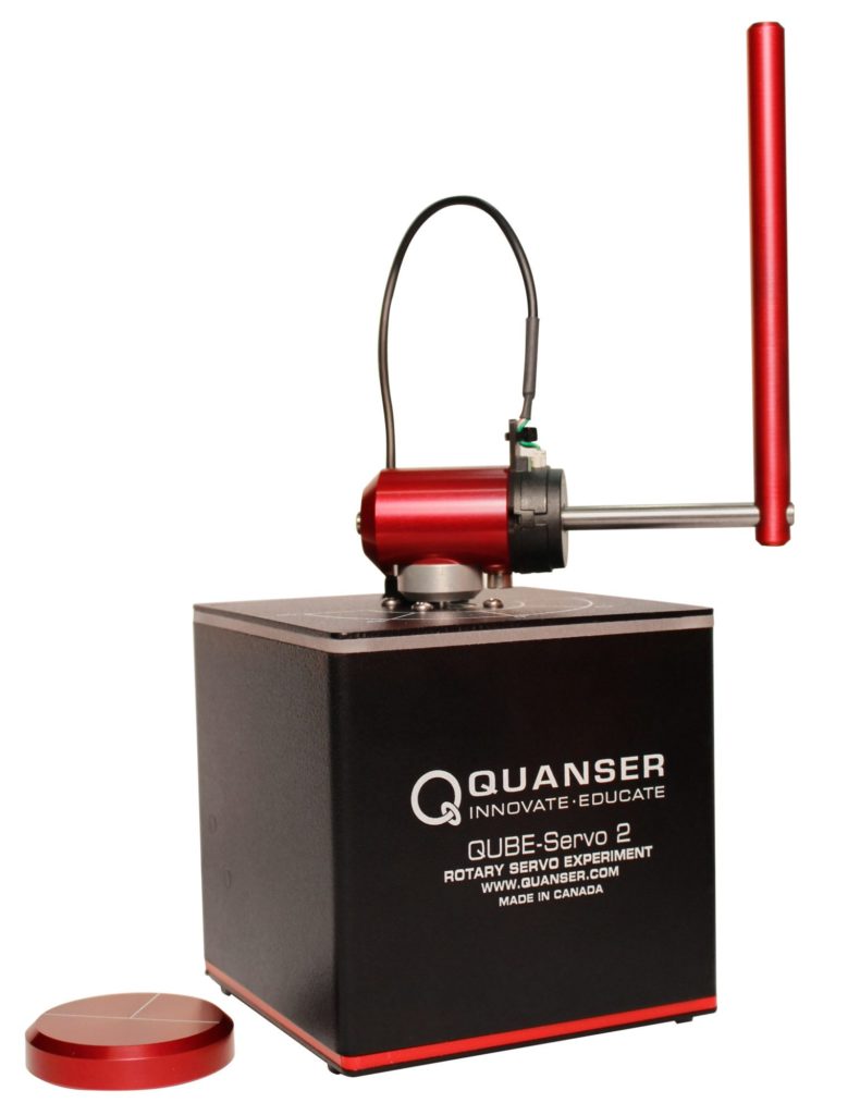
The Quanser Coupled Tanks, shown below, is a reconfigurable, nonlinear process control experiment that is not easy to control. In the supplied courseware, we go through the design of a PID and feed-forward controller (PID+FF) to control the level of water in the tank. While it does perform well, the PID+FF control follows a model-based design approach. If the model does not accurately represent the system, then the controller may not perform adequately and as expected. For more information about the control challenges and design using PID+FF, please see my previous blog post.
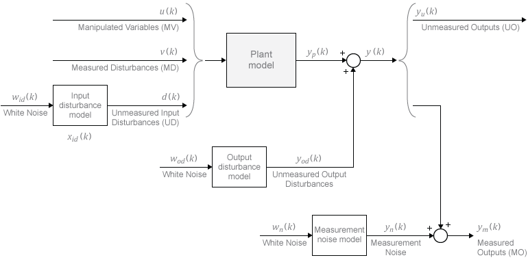
Model Predictive Control (MPC) is an advanced adaptive type control method that requires less knowledge of the plant dynamics. The MathWorks Model Predictive Control Toolbox makes it easy to design and implement MPC controllers. The MPC design starts with defining the various input and output signals and their limits. Figure 1 illustrates the plant model signals used in the MPC controller. You still need to have a representative model, but because of its adaptive nature, less control design is required and it can compensate more for effects such as parameter uncertainties and disturbances.
Coupled Tanks MPC Design
In this section, the step-by-step MPC control design procedure to control the level of water in Tank 1 of the Coupled Tanks system is outlined.
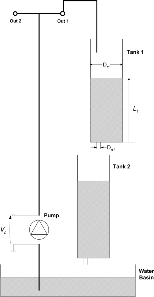
The input, or Manipulated Variable (MV), is the pump voltage and the output is the measured level, denoted as the Measured Output (MO). We could also define the disturbance tab as an Unmeasured Output (UO). The tank level is limited between 0 to 25 cm and the tank voltage from 0 to 22 V. Given this, we can choose the limit and scaling for MO and MV.
- We have a fairly representative nonlinear model of the Coupled Tanks system. In order to use the Linear MPC implicit control, the model is first linearized about the operational point V_p0 and L_10, where V_p0 is the voltage needed to maintain the level at L_10 = 15 cm. The resulting linear equations of motions are then represented as a transfer function object, using the Control Systems Toolbox™.
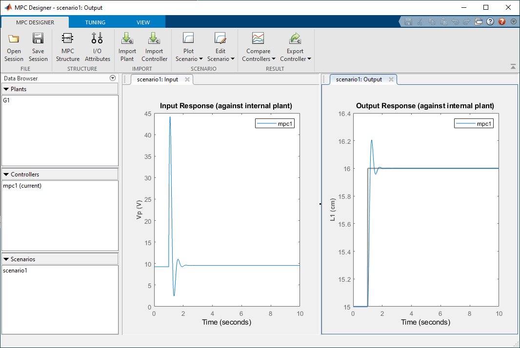
- Run mpcDesigner in the MATLAB Command Window.
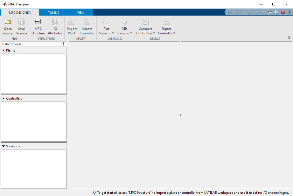
- The Transfer Function model of the Coupled Tanks is defined as object G1 in the MATLAB Workspace. To import the model into the MPC Designer, click on the MPC Structure button.
- Select the G1 model and set the sample time, for now, to 0.01 seconds. Click on Define and Import. As expected, this includes one Manipulated Variable (MV) – the pump voltage – and one Measured Output (MO) signal – the level of Tank 1.
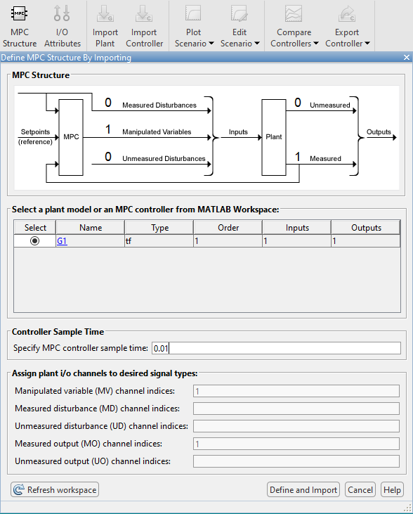
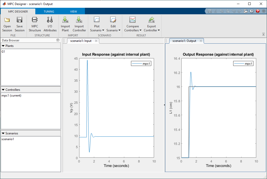
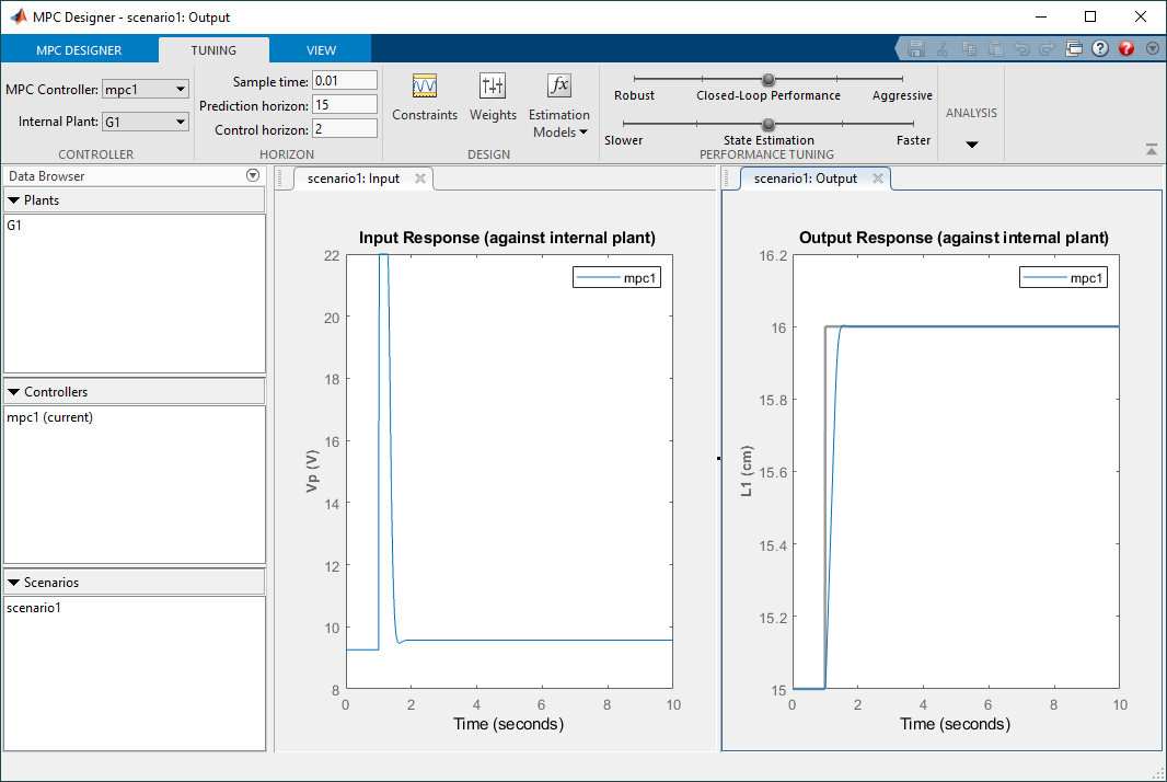
- As shown below, this is already showing an input and output response. The MPC Controller is already working, and in addition, has a fairly good response.
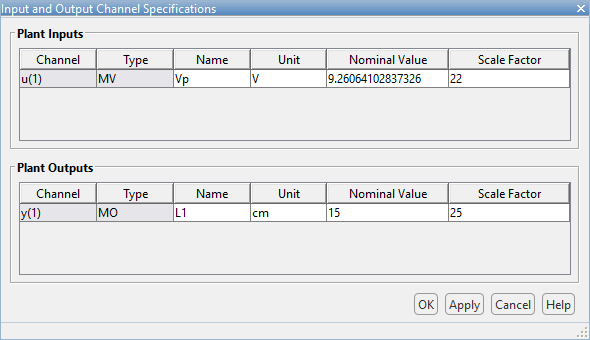
- Click on the I/O Structure icon in the toolbar to define names, units, nominal values (operating point used for linearization), and the scale factor. The scale factor specifies the range of the variables. In this case, the tank level is limited between 0 and 25 cm and the pump voltage from 0 to 22 V. The nominal voltage of 9.26V is the voltage needed to to keep the water level of tank 1 at 15 cm.
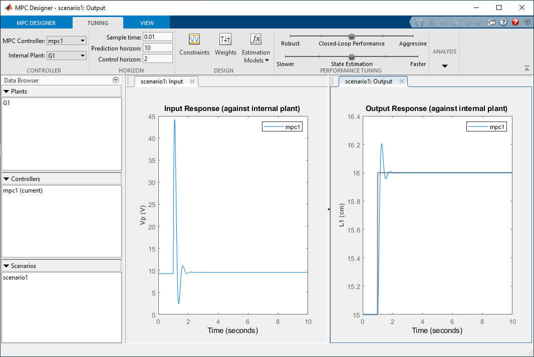
- The main MPC Tuning parameters are sample time, prediction horizon, and control horizon.
- The sample time, T_s, is set to 0.01 sec. Given the open loop time constant is over 10 sec, this sample time should be more than enough. Faster sample times can result in better response (depending on the system) but are more computationally intensive.
- Prediction horizon, p, adjusts the foresight of the MPC controller. Larger p results in better performance but at the expense of additional computation time.
- Control horizon adjusts how fast the MPC controller will optimize the control. The default it is 2 and based on the adequate response already obtained, is left at that value.
- While the overshoot is a bit high at p=10, it decreases when p = 15 as shown below.

- The Constraint imposes the min/max values on the manipulated variable (MV) input and measured output (MO) variables as well as rate limitations.
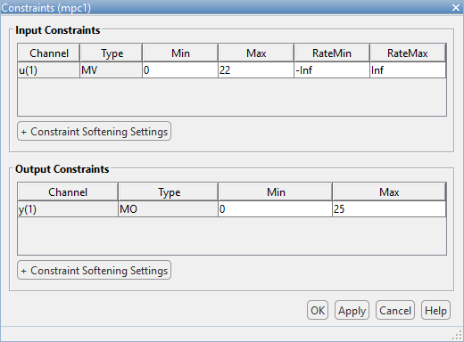
- Defining these constraints allows the MPC to be further optimized and, as shown below, lowers the overshoot in the response.
- Further adjustments can be made using the Weights.
- Finally the Export Controller function is used to export the MPC controller as a MATLAB Script. Based on the parameters chosen, the script creates a MATLAB MPC object that is used by the MPC Controller block in Simulink. It also allows us to make some final adjustments based on the response we obtain in the Simulink model.
Model Predictive Control – Running the Simulation
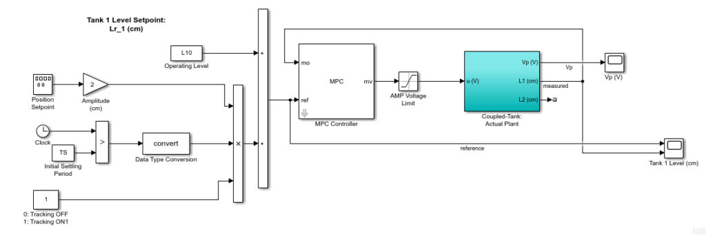
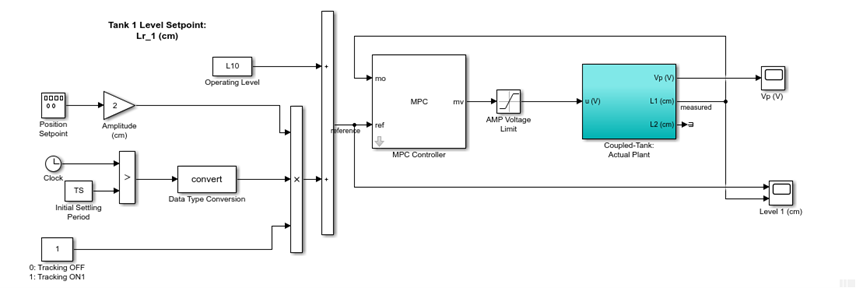
The Quanser Coupled Tanks system comes supplied with full documentation, including courseware for students and instructors, as well as the Simulink models and MATLAB scripts used to design and simulate the PID+FF control. The Model Predictive Control designed above is implement using the MPC Controller block from the Model Predictive Control Toolbox. The supplied PID+FF based Simulink model was modified to include the MPC Controller block as shown below.
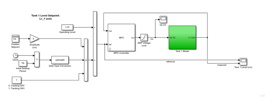
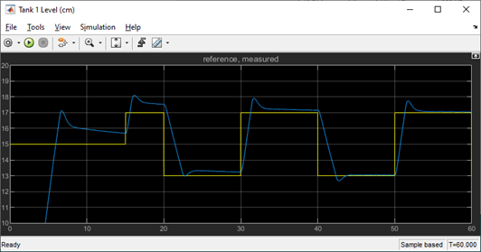
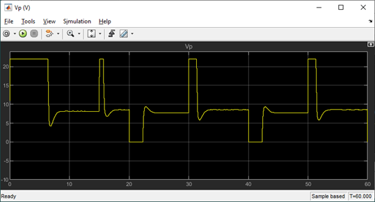
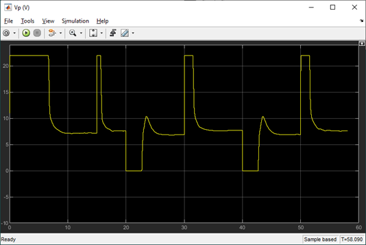
The Simulink diagram includes a nonlinear model of the Coupled Tanks in order to obtain a more representative response of the actual plant when testing controllers. The response obtained when simulating the MPC controller is given in the scopes below.
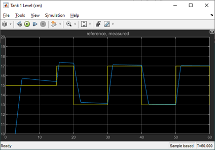
As shown in the Tank 1 Level scope, the tracking response improves as the simulation is running, i.e. the steady-state error decreases after each cycle. Compared to the PID+FF control supplied in the standard material, the MPC response has less settling time and overshoot. All done using a slower sampling rate, 100 Hz vs. 500 Hz, and less control design effort.
Model Predictive Control – Running it on the Virtual System
The QLabs Virtual Coupled Tanks system includes a high-fidelity nonlinear dynamic model of the Coupled Tanks. As done in the simulation, the MPC designed above is implemented on the Virtual Experiment using the MPC Controller block from the Model Predictive Control Toolbox (by modifying the PID+FF based Simulink model supplied).
The response when running the MPC controller on the Virtual System is shown in the Simulink scopes below. As in the simulation, the water level tracking with MPC improves over time. By the third cycle, the steady-state error goes down to 0.06 cm.
The response is comparable with the PID+FF control running on the virtual experiment. The MPC has a faster response and better settling time but has a larger overshoot. The overshoot could probably be decreased by increasing the prediction horizon. Again, all done using lower sampling rate and less time designing the controller.
You may notice that this response is different from the simulation results obtained in the MPC Designer application. Recall that the MPC Designer used the linearized model where, in this case, the Coupled Tanks Virtual model is nonlinear and includes additional effects such as pressure sensor noise and pump delays.
Model Predictive Control – Running it on the Hardware
Finally, the Simulink model below implements the MPC controller designed on the physical Quanser Coupled Tanks. The MPC control designed is implemented using the MPC Controller block from the Model Predictive Control Toolbox, similarly as in the virtual plant, and the hardware interface and deployment is done using the QUARC Real-Time Control software.
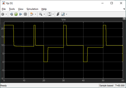
Here are some example results of the level control and corresponding pump voltage.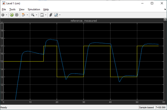
Compared to the virtual experiment, there is a larger steady-steady error when running the MPC on the hardware. However, the steady-state error improves as the controller is running and there is no overshoot. The response is slower (i.e. larger peak and settling time), but this could be improved by increasing the prediction horizon and/or tuning the MPC weights.
Future Work
Model Predictive Control (MPC) can be used on a variety of systems. There are also different types of MPC controllers. For the Coupled Tanks, we designed and implemented the standard implicit MPC control. In the future, we plan on exploring other types of MPC that are available the MathWorks Model Predictive Control Toolbox for Simulink:
| Explicit MPC Controller | Nonlinear MPC Controller | Gain Scheduled | Adaptive MPC |
| Less computationally intensive by using precomputed solutions. | Similar to the linear implicit MPC controller, but it allows nonlinear prediction models, cost, and constraints. | Switches between different MPC controllers designed for different operating points. | Updates the MPC controller in real-time. Typically used for systems with complex dynamic, e.g. time-varying systems. |
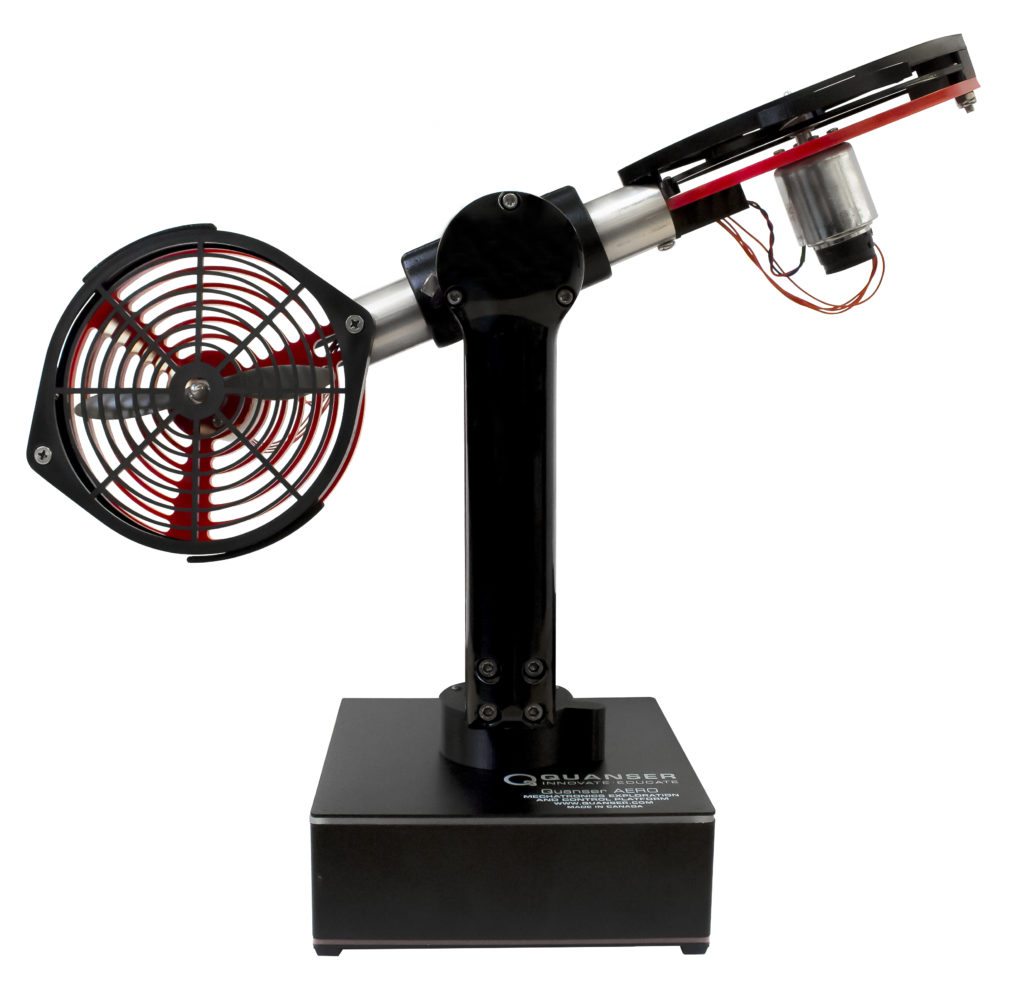
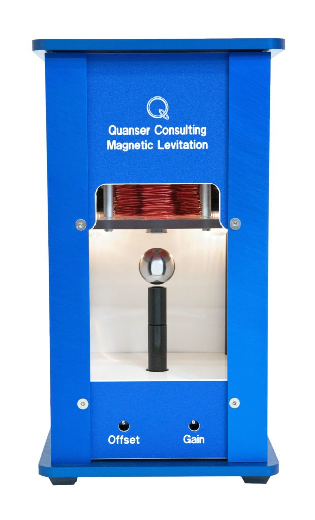
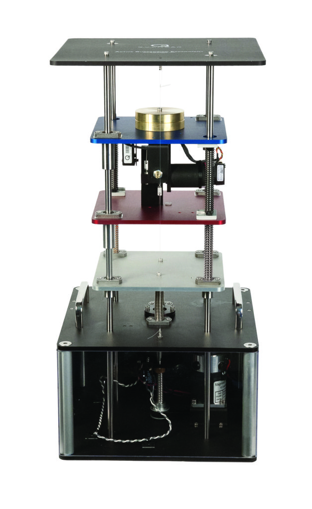
| The QUBE-Servo 2 Inverted Pendulum system can benefit from a fast model predictive control at higher sampling rates. | The Quanser AERO in the 2 DOF configuration is both nonlinear and has coupled cross-torque effects between the two rotors. | The electromagnetic force acting on the ball of the Quanser Magnetic Levitation is nonlinear and changes exponentially depending on the air gap between the ball and magnet. | Optimizing the ride-comfort of the Active Suspension for different road profiles. |
 |
 |
 |
 |
Resources
Please visit the MathWorks website for more information on the Model Predictive Control Toolbox:
- Model Predictive Control Toolbox video series: https://www.mathworks.com/videos/understanding-model-predictive-control-part-1-why-use-mpc–1526484715269.html?s_tid=srchtitle
- Model Predictive Control Toolbox homepage: https://www.mathworks.com/products/model-predictive-control.html