

PID is hands-down, the most popular type of control method used in industry. However, there are many variations of PID controllers and different design methods to find the proportional, derivative, and integral gains. In this blog we show how fast and effective the Simulink® Control Design™ Toolbox PID Tuner App can be used to control the level of water in the nonlinear Quanser Coupled Tanks system.
Why use PID Tuner?
Proportional-derivative-integral (PID) control is the most widely implemented control strategy in industry. Mostly due to the widespread use of Programmable Logic Controllers (PLC) in automation and process control industries, which commonly use PID control.
At Quanser, we use PID-based control for many of our 60+ systems. PID design is typically done on the linear model of the system and to meet certain frequency-domain or time-domain requirements, such as peak time and overshoot.
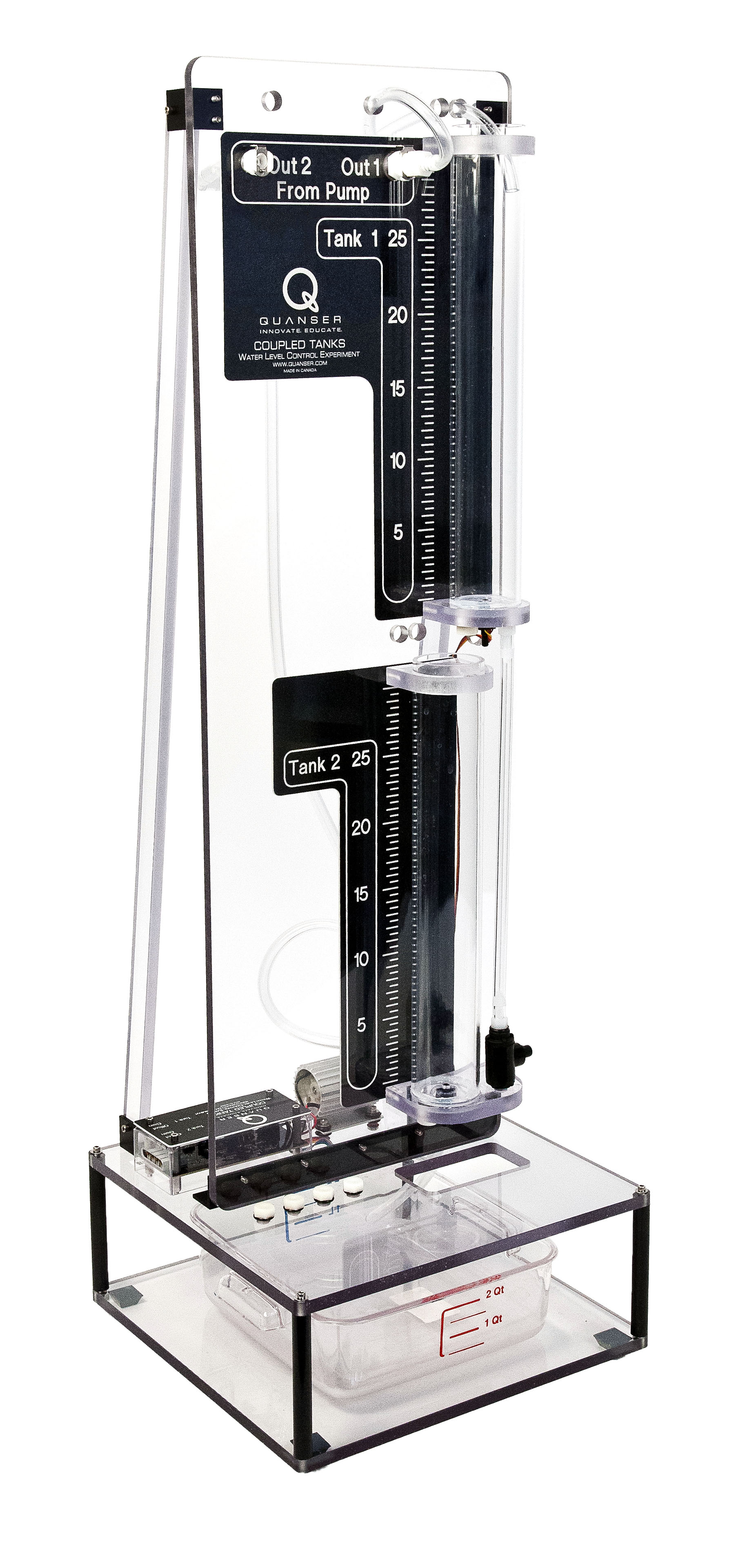
The Quanser Coupled Tanks, shown below, is a reconfigurable, nonlinear process control experiment that’s not easy to control. In the supplied courseware, we go through the design of a PID and feed-forward control (PID+FF) to control the level of water in the tank. While it does perform well, the PID+FF control follows a classical model-based design approach where the nonlinear model is first linearized by-hand, the feed-forward gain is found from the system dynamics, and the PID gains are calculated based on second-order time-domain requirements.
For more information about the control challenges and design using PID+FF, please see this previous blog post.
This type of system therefore requires a significant amount of modelling and control design. Instead, here we investigate using Simulink Control Design Toolbox to find PID gains that meet certain performance criteria. In some ways, this is more in-line with how industry uses PID auto-tuning software that is often supplied with PLCs.
Linearization
The PID Tuner App uses a linear model to compute the PID gains. The Coupled Tanks is a nonlinear system. Typically, we would linearize the nonlinear model by-hand about a certain operation point, in this case when the tank 1 level is at the 15 cm mark. Instead of doing this manually, we can instead use the Simulink Linearization tools to find the linear model.
The procedure below outlines our design steps. You can also watch the below video.
Setup the Linearization Points
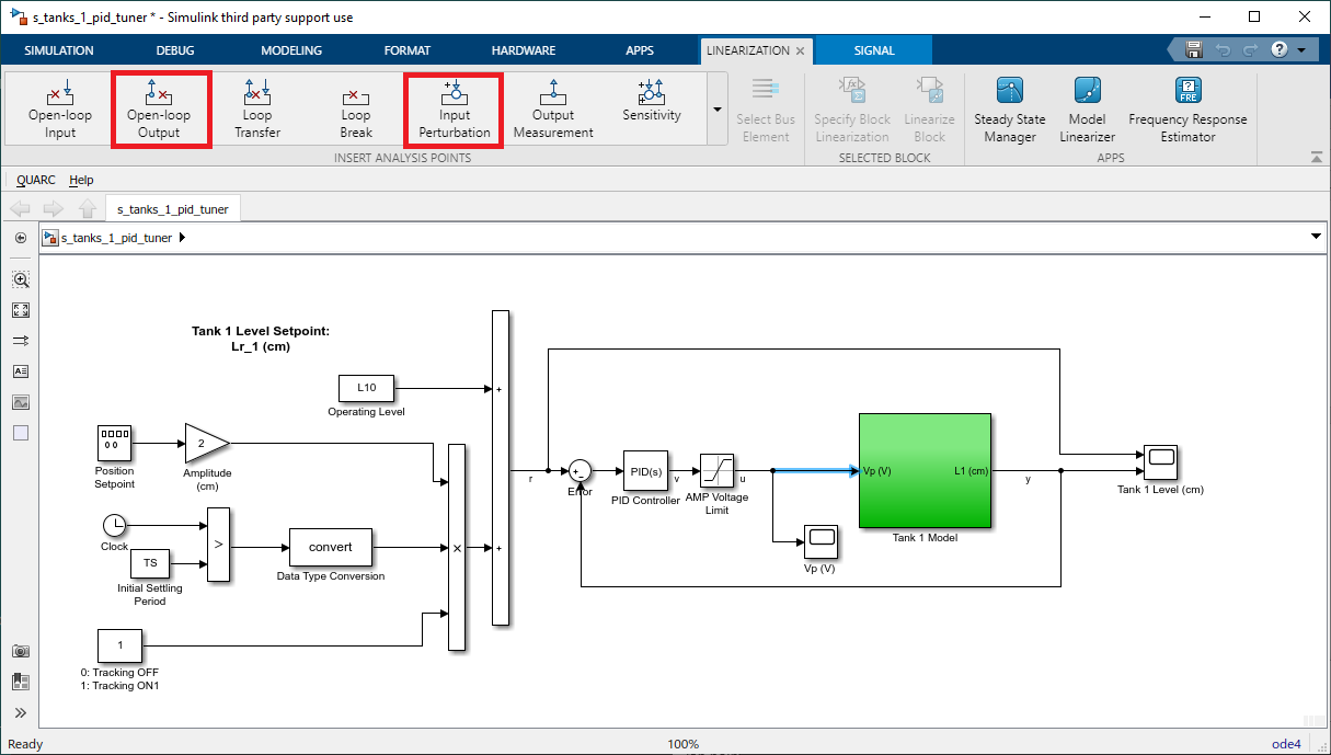
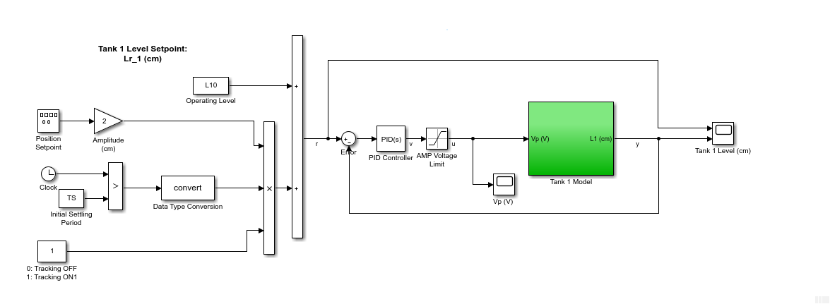
The Simulink model simulates the Quanser Coupled Tanks using a nonlinear model, defined in the Tank 1 Model subsystem. The PID control is implemented using the Simulink PID Controller block.
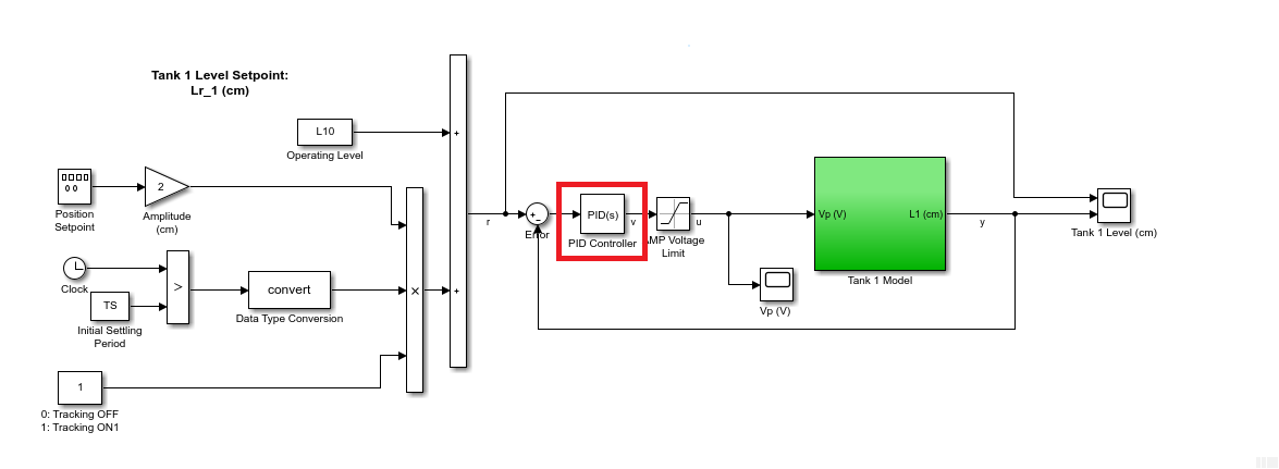
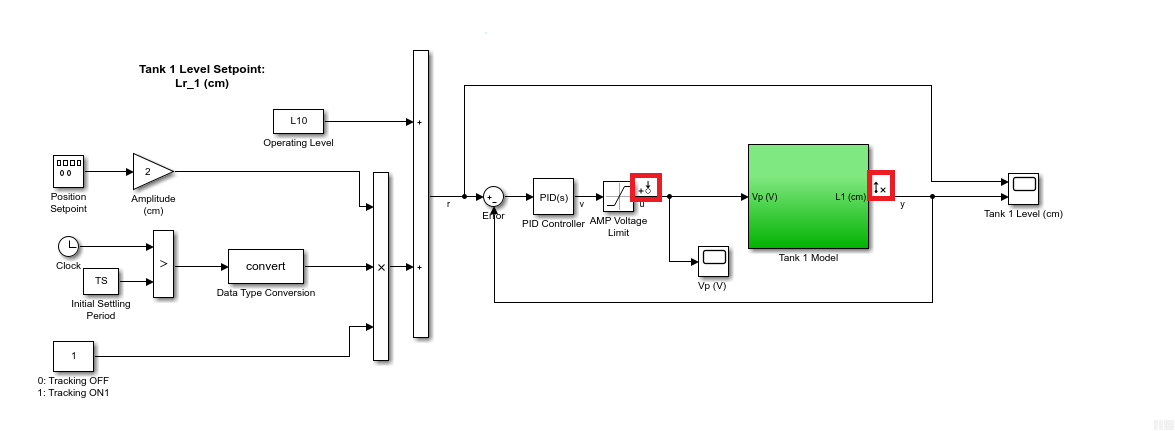
- The input to the plant, i.e. the pump, is defined as an Input Perturbation. The output of the plant is the water level of tank 1, which is measured using a pressure sensor, is defined as an Open-loop Output.
 .
. - The Simulink model with the linearization points defined is shown below.
- With the linearization points defined, click on Model Linearizer button to load the application.
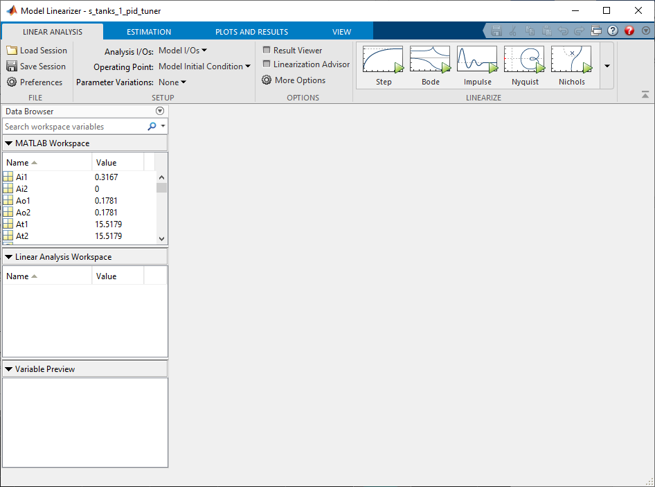
Model Linearizer Configuration
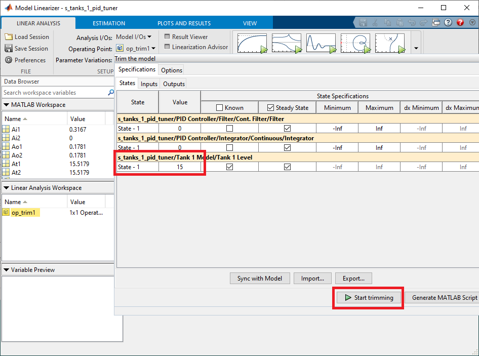
- The Analysis I/Os setting is defined as the Model I/Os we have just defined above. The Operating Point needs to be changed because we will be controlling the water level about the 15 cm mark. In order to define this operating point for the linearization, go to Trim Model.
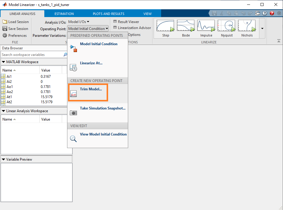
- Set the value of State-1 in the s_tanks_pid_tuner/Tank 1 Model/Tanks 1 Level/ row to 15 cm.
- Click on Start trimming. This will create an operating point called op_trim1. The Operating Point field in the toolbar is automatically set to the new op_trim1 operating point that was just defined.
Linearize Plant
- We can now proceed with the linearization and view the step response plot by clicking on the Step button.
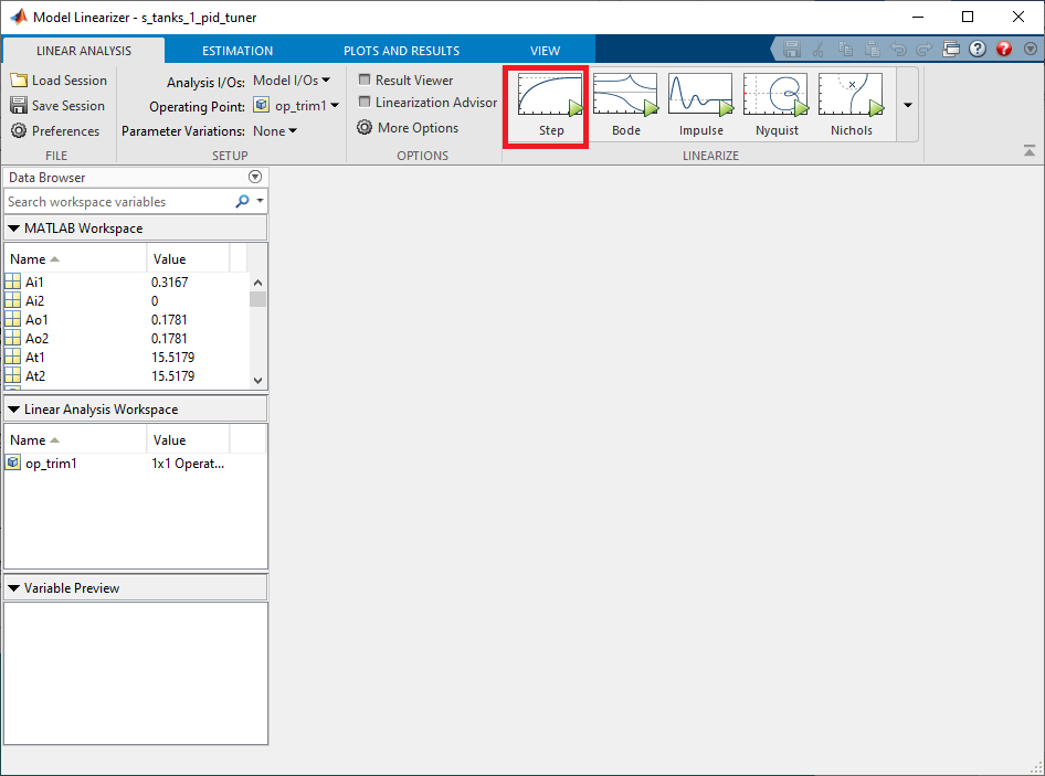 This creates a linear model called linsys1.
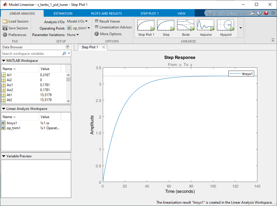
- We can rename linksys1 to tanks1_mdl_lin and view the corresponding transfer function model that it generated by clicking on the Plots and Results tab and clicking on the Results Viewer button.
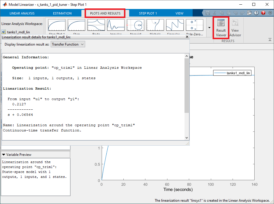
- Now that we have our linear model, we can drag the tanks1_mdl_lin object to the MATLAB Workspace in order for the model to be available to the PID Tuner.
Running the PID Tuner
- Double-click on the PID Controller block to open its dialog.
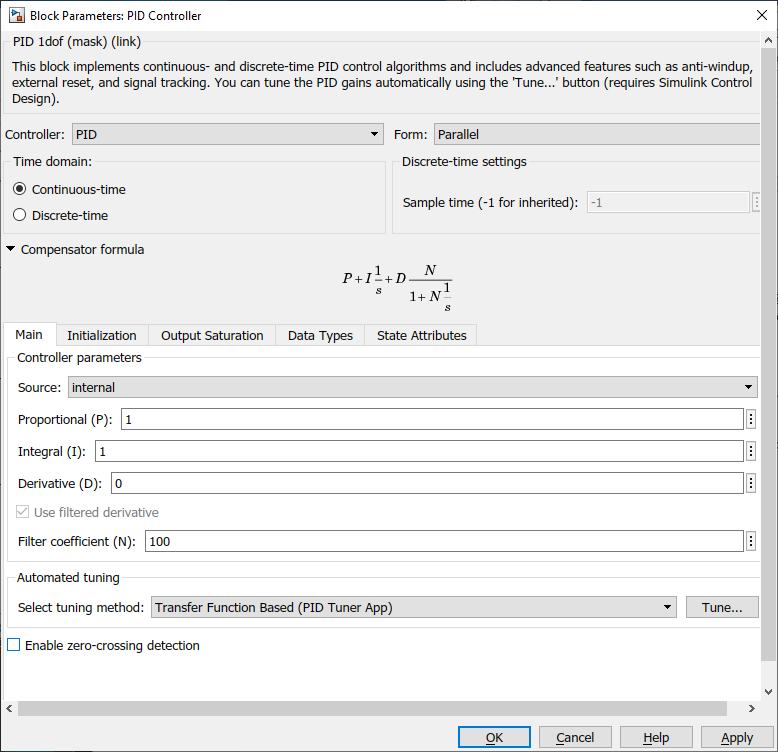
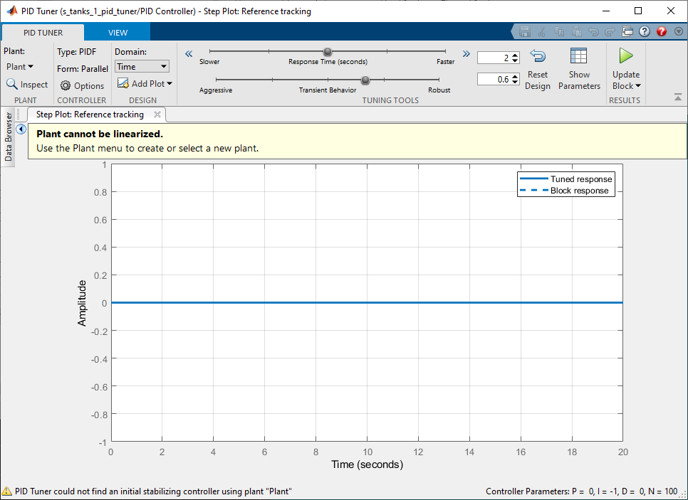
- Select the Transfer Function Based (PID Tuner App) tuning method and click on the Tune. Note: it may prompt an error that it cannot linearize the plant. We can ignore this since we have already done the linearization and have a linear model of the system.
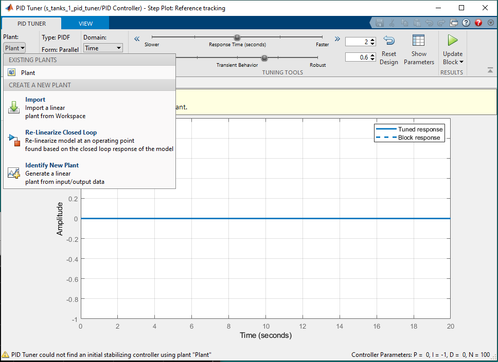
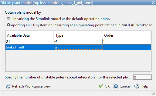
- To use the plant we linearized, go the Plant section in the top-left corner and select Import.
- Select the tanks1_mdl_lin variable we created.
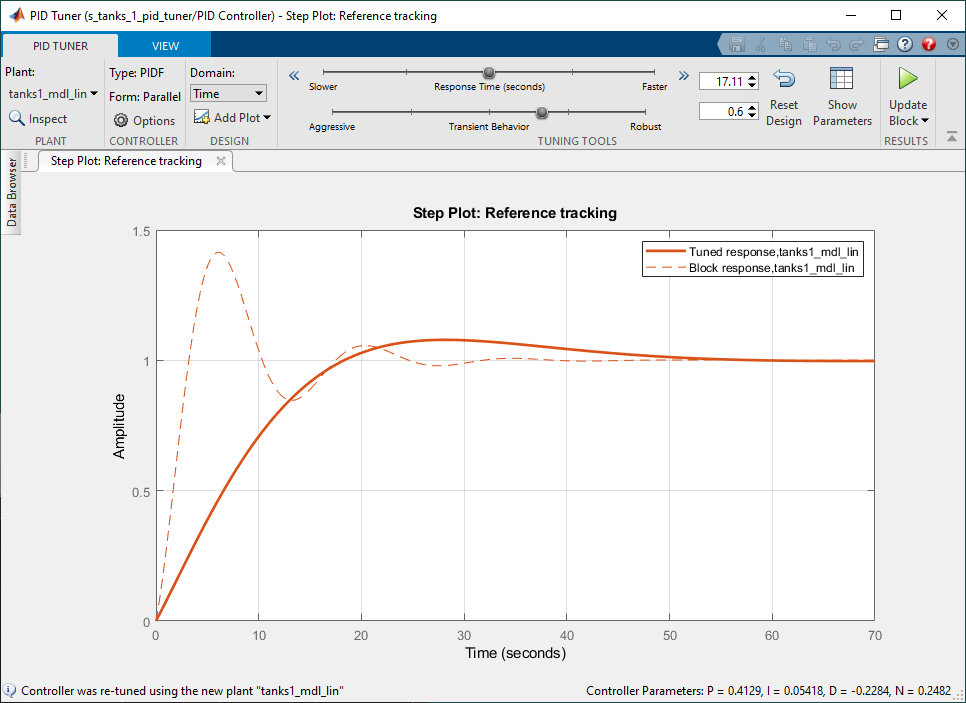
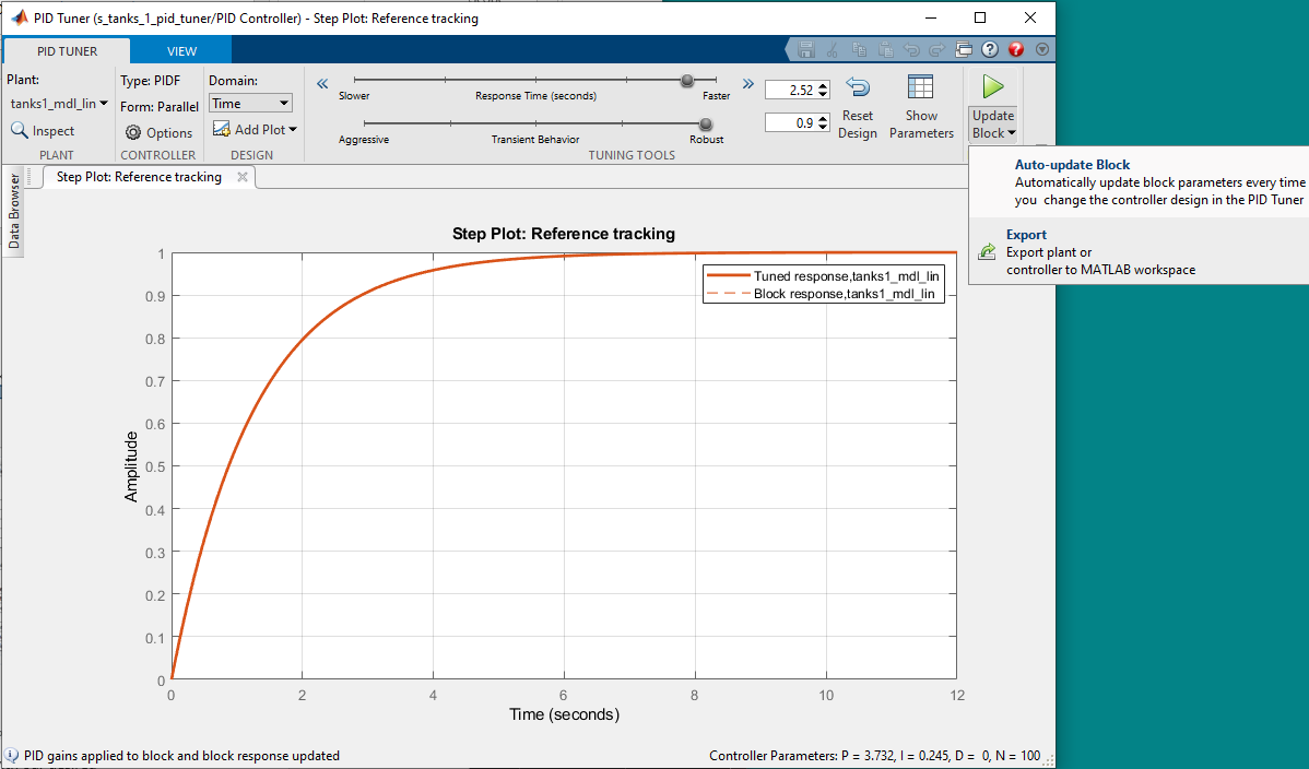
- The Step Plot: Reference Tracking figure shown below displays the tracking response of two systems:
- Block response: Response using the linear model and the PID gains that are set in the PID Controller block in the Simulink model.
- Tuned response: Response using the linear model and the gains found with the PID Tuner.
- As shown, the PID tuner has already found a set of gains that gives us reasonable initial tracking response.
- Our design goals for controlling the water level of the tank are:
- Maximum percent overshoot of 5%
- Settling time less than 5 s
- Steady-state error less than 0.1 cm
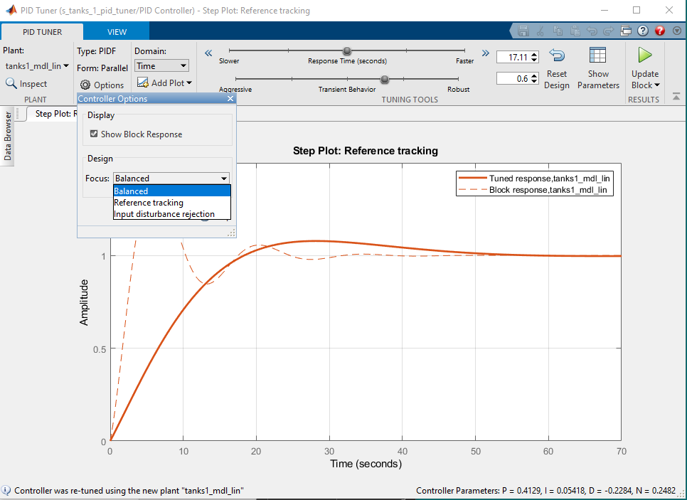
- Click on the Options button. The PID Tuner can be optimized to different design goals: Reference Tracking, Input Disturbance Rejection, or the Balanced approach. Here we select Reference Tracking.
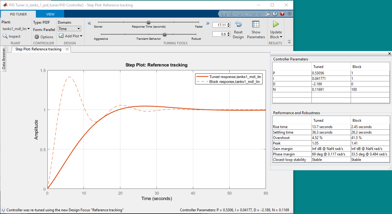
- Click on the Show Parameters button. This displays the PID gains generated as well as the resulting overshoot and settling time obtained in the linear simulation.
- Adjust the Response Time and Transient Behavior sliders until we get our desired response. The Transient Behavior was increased to 0.9 to reduce the overshoot of the response. The Response Time slider was then set to 2.52 s to get a settling time of 4.93 s.
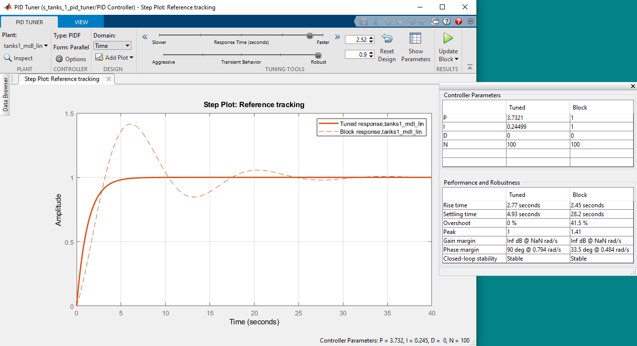
- Based on the linear-model based simulation, the Tuned response complies with our desired specifications. We can now test this again using the nonlinear plant to get a more realistic response at a different operating range. Click on the Update Block button to set the PID Controller block gains in the Simulink model to the tuned ones just found. We can also export this as a MATLAB Transfer Fcn object, e.g. C, in order to use this in other Simulink models.
Simulink Coupled Tanks Nonlinear Simulation
Go back to the Simulink model with the nonlinear model defined, in the Tank 1 Model subsystem, and with the tuned PID gains set in the PID Controller block.
Running the Simulink model based on the nonlinear model of the Coupled Tanks using the tuned PID gains, we get the following response.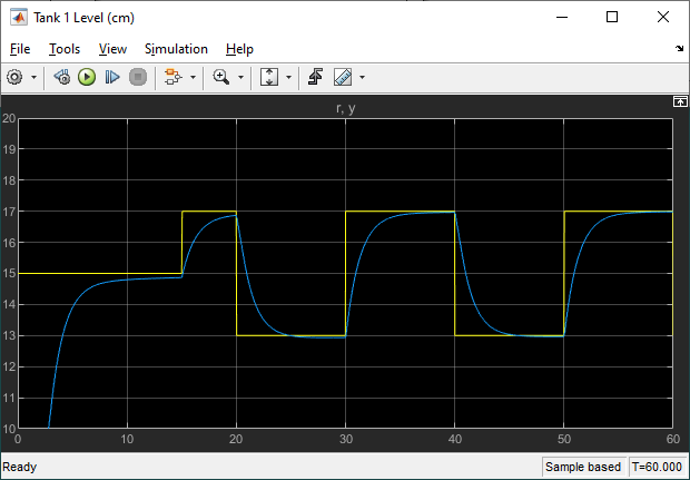
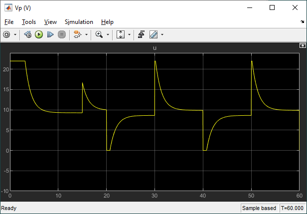
The resulting settling time is 3.26 s with no overshoot or steady-state error, thus complying with our design goals. Given that we have a set of gains matching our requirements in simulation, we can move on to the Virtual Twin of the Coupled Tanks.
QLabs Coupled Tanks Virtual Experiment
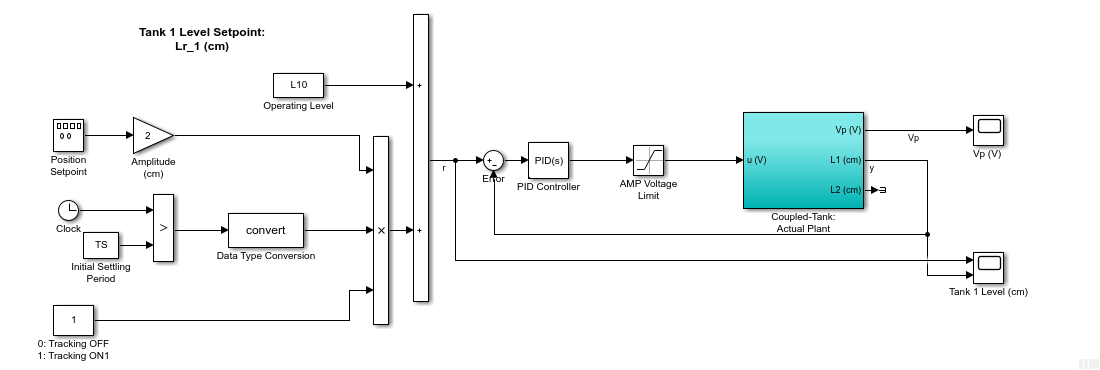
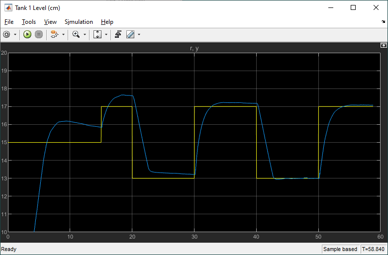
The QLabs Coupled Tanks Virtual Experiment uses a higher-fidelity nonlinear model that includes pump actuator delays, sensor noise, and so on. The Simulink model shown below is configured to interface to our QLabs Virtual Coupled Tanks Experiment. Here we show the system when it is almost complete with the 60 s cycle simulation.
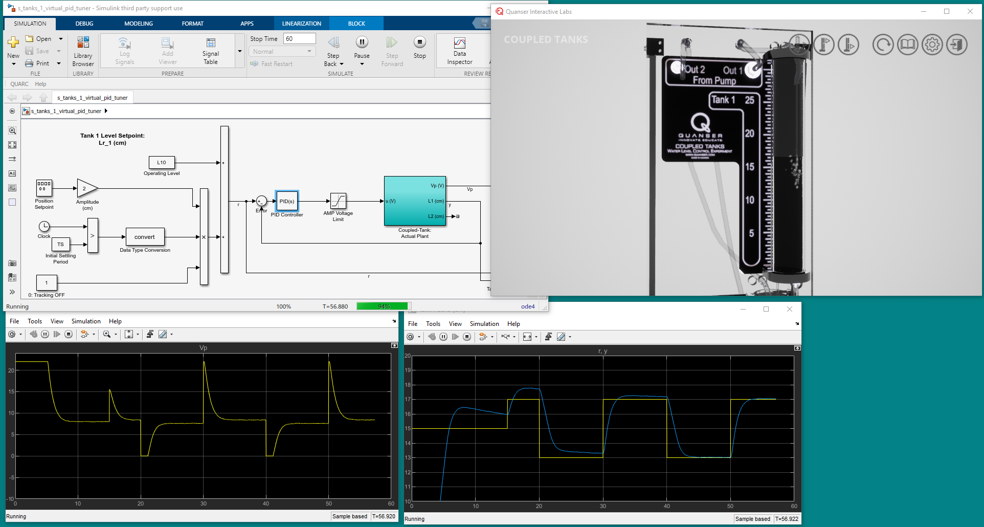
The PID Controller gains are set to the values found using the PID Tuner previously. This was done by just typing in the compensator Transfer Fcn object C that was exported from the tuner.
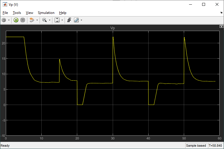
Here is the response we obtain when running the PID control tuner gains on the virtual twin.
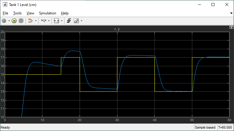
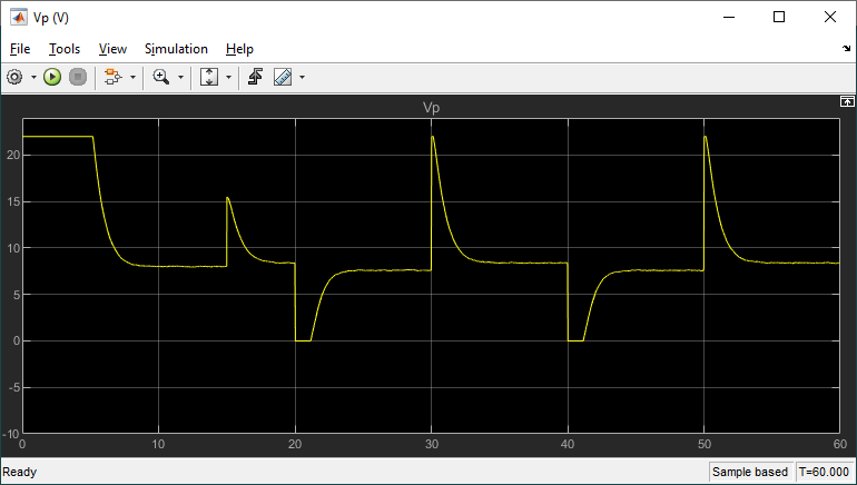
Looking at the last cycle where the step starts at the 50 s mark, we have a 2% settling time of 2.18 s, no overshoot, and a steady-state error of 0.03 cm. Our design requirements are met on Virtual Twin of the Coupled Tanks and we are now ready to test this on the actual hardware.
You can watch the video below to see this in action.
You may have noticed that we actually obtain a better, i.e. shorter, settling time in both the nonlinear Simulink simulation and the QLabs Virtual Experiment compared to the PID Tuner simulation. The gains that were designed in the PID tuner to get a settling time of 5 s were based on the ideal linear simulation. The linear simulation is also running about a different operating point, showing the step response of the water tank going from 0 to 1 cm. In the other simulations, we are controlling the system at about 15 cm. As mentioned earlier, the model used in the QLabs Virtual Experiment includes dynamics that more closely resemble the hardware. For instance, the pump inflow rate changes depending on the voltage applied. These are some reasons for the discrepancy.
Coupled Tanks Hardware
The Simulink model shown below implement a PID control on the Quanser Coupled Tanks hardware using the Quanser QUARC Real-Time Control software.
The scopes below show the actual system response.
Here we have a steady-state error of 0.08 cm, no overshoot, and a settling time of 2.7 s. The settling time meets our design goal of being under 5 s. Success! The PID Tuner found gains that work across all the simulations and on the actual system.
You can watch the video below to see this in action.
Result Summary
Here’s a summary of the results for the Coupled Tanks simulation using an idealized nonlinear model, the QLabs Coupled Tanks Virtual Experiment, and the actual Quanser Coupled Tanks hardware.
| Design Goals | Simulation | Virtual Model | Hardware | |
| PID Gains | P = 3.73 I = 0.245 D = 0 N = 100 |
P = 3.73 I = 0.245 D = 0 N = 100 |
P = 3.73 I = 0.245 D = 0 N = 100 |
|
| Percent Overshoot (%) | 5% | 0% | 0% | 0% |
| 2% Settling Time (s) | 5 s | 3.60 s | 2.18 s | 2.70 s |
| Steady-state error (cm) [absolute value] | 0 | 0.02 cm | 0.03 cm | 0.08 cm |
The integrator does a good job at minimizing the steady-state error in all cases to less than our 0.1 cm design goal. Despite not having any derivative, the tuner found a set of PI gains that obtained no overshoot. The settling time matches our design goal of being less than 5 s. Quite impressive given the amount of design time compared to doing this manually.
Final Thoughts
The Simulink Control Design Toolbox has been around for many years now. It’s easy to use and effective. The Model Linearizer App saves us the time from having to linearize the nonlinear model by hand. As discussed earlier, in the original design the model was linearized manually and the PID and feed-forward gains were found to match a set of desired requirements. This is a classic approach and it does achieve great results. However, the response we got using the PID Tuner App was very favorable as well and it matched our desired specifications – and it did most of the work for us!
Resources
See the PID Controller Tuning in Simulink document on the MathWorks Help Center: https://www.mathworks.com/help/slcontrol/gs/automated-tuning-of-simulink-pid-controller-block.html