
The Quanser Magnetic Levitation shown below is a one-dimensional magnetic levitation system. It has an optical ball position sensor and a current sensor to measure the current in the electromagnet coils.
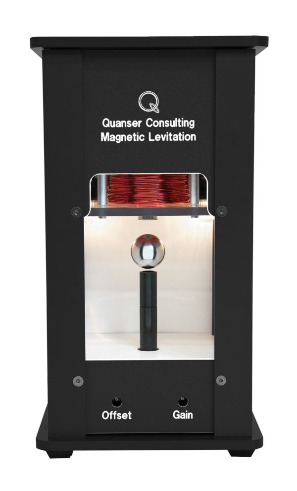
The Maglev system is a challenging control systems application for several reasons:
- Nonlinear dynamics.
- Ball levitation is unstable.
- Uncertainties: Electromagnetic force acting on the ball changes quickly depending on the air gap, i.e., distance between the ball and the electromagnet, and the current applied in the coils. The force can also vary over time, i.e., magnet coil heats up and causes the inductance to increase.
- Actuator dynamics: Large inductance of the electromagnet causes a huge delay in the actuator response. As a result, a current control is needed. In the ball position control design, we assume that the current in the coils equals the current commanded. However, even with the current control there is always a slight delay.
- Sensor noise: Although small, there is still some noise in the current and ball position sensors.
Given the inherit nonlinear dynamics and uncertainties, robust control techniques are often used in magnetic levitation and other similar applications. Here we show how to use the MathWorks® Robust Control Toolbox™ to define an uncertain variable and use the Control System Tuner app to tune a robust controller that can help compensate for the variance in the magnet force constant and the other uncertainties that are not accounted for.
Ball Position Model
The Quanser Magnetic Levitation System can be modeled as follows.
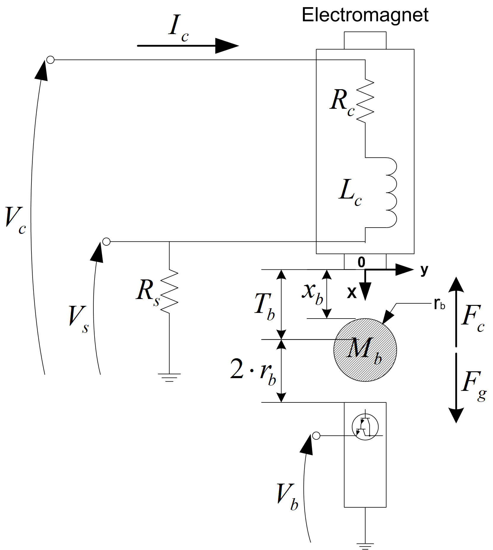
Using the notation and conventions shown above the attractive force generated by the electromagnet and acting on the steel ball can be expressed by
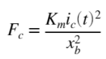
where ![]() is the air gap between the ball and the face of the electromagnet and
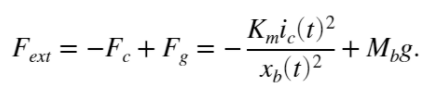
is the air gap between the ball and the face of the electromagnet and ![]() is the electromagnetic force constant. The force produced by the electromagnet is proportional to the square of the current and inversely proportional to the air gap (i.e., ball position) squared. The total external force acting on the ball is from the electromagnetic and gravitational forces
is the electromagnetic force constant. The force produced by the electromagnet is proportional to the square of the current and inversely proportional to the air gap (i.e., ball position) squared. The total external force acting on the ball is from the electromagnetic and gravitational forces
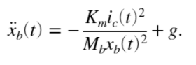
Resulting in the following nonlinear equation of motion (EOM)
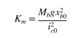
The force constant can be derived from the measured current and air gap position. If the ball is maintained at a fixed position, , then a certain current is needed to stabilize it to that point![]() ,
,
Variable Electromagnet Force
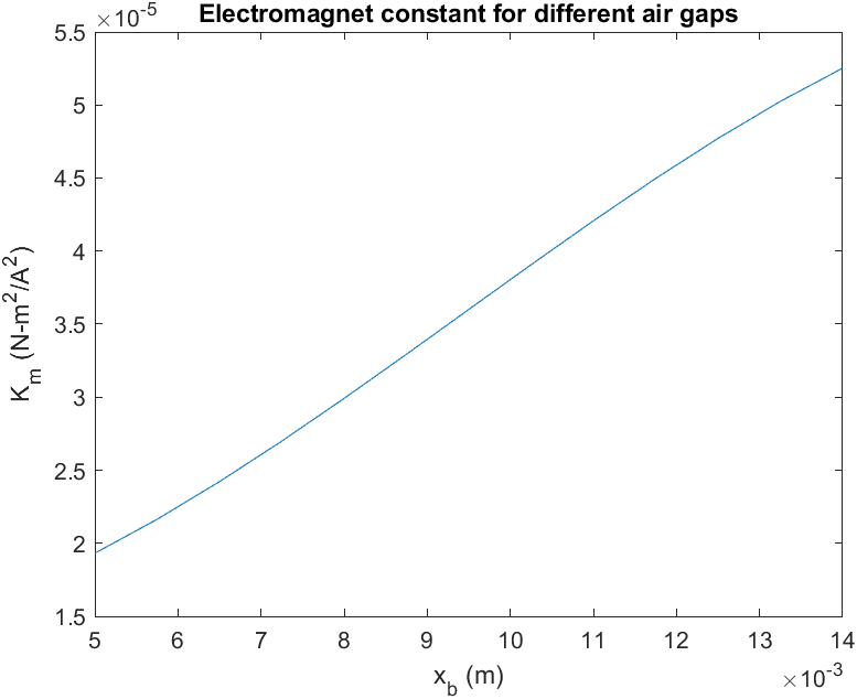
The ball position model uses a fixed electromagnet parameter, ![]() . However, based on this model the electromagnet parameter changes depending on the air gap. This data was collected by looking at the current needed to stabilize the ball at different air gap positions.
. However, based on this model the electromagnet parameter changes depending on the air gap. This data was collected by looking at the current needed to stabilize the ball at different air gap positions.
The electromagnet constant can be defined as an uncertain parameter in MATLAB and used in our robust tuning design.
% Define electromagnet force constant as uncertain parameter
Km_un = ureal('Km',Km,'range',[min(Km_est) max(Km_est)]);
We can design a PID control based on this uncertain variable and see how it affects the ball position response.
Linearize Plant with Uncertain Parameters
The nonlinear plant is defined in a Simulink model as shown below.
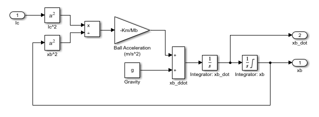
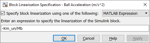
The model is linearized using the uncertain electromagnet constant. To do this, go to Linear Analysis | Specify block linearization option in the Ball Acceleration block and define the gain using the Km_un parameter.
The linearization is performed about the operating air gap, xb0, and current, ic0. The ranges of the states are defined based on the min/max current of the electromagnet, 0 to 3 A, and the ball travel range, 0 to 14 mm.
% Open Simulink model with nonlinear model of Maglev
mdlPlant = 'maglev_model';
load_system(mdlPlant);
open_system([mdlPlant '/Maglev Nonlinear Plant']);
%
% Specify linearization input and output points.
io(1) = linio([mdlPlant '/Ic'],1,'openinput');
io(2) = linio([mdlPlant '/Maglev Nonlinear Plant'],1,'openoutput');
% Set operating point and min/max values of states
opspec = operspec(mdlPlant);
% ball position state is known
opspec.States(1).Known = true;
opspec.States(1).x = xb0;
opspec.States(1).Min = 0;
opspec.States(1).Max = Tb;
opspec.Inputs(1).u = ic0;
opspec.Inputs(1).Min = 0;
opspec.Inputs(1).Max = IC_MAX;
%
% Compute operating point using these specifications.
options = findopOptions('DisplayReport',false);
op = findop(mdlPlant,opspec,options);
%
% Obtain the linear plant model at the specified operating point.
GxbIc = linearize(mdlPlant,op,io);
GxbIc.InputName = {'u'};
GxbIc.OutputName = {'y'};
% View transfer function when using nominal value.
tf(GxbIc)
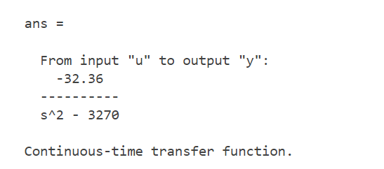
As shown, the transfer function has an unstable pole.
Ball Position Control Design
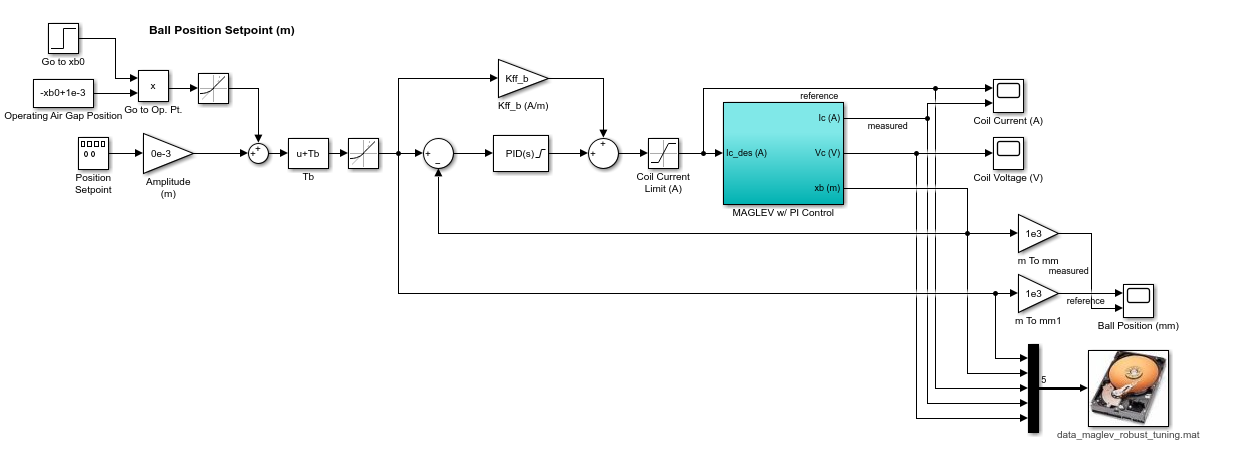
The ball position is controlled using a PID and feed-forward design.
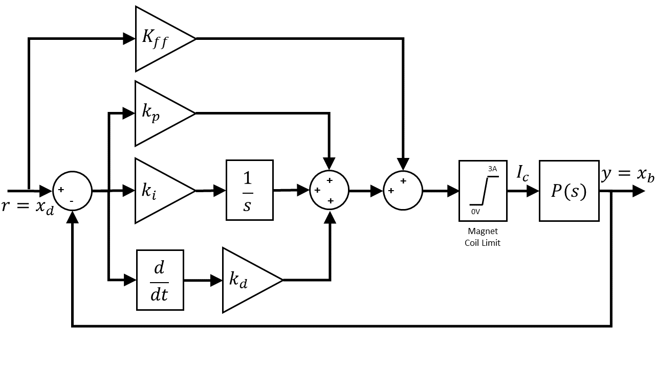
The PID gains are found through the MATLAB Control System Tuner app. Because there is a small amount of noise in the ball position sensor, a first-order filter is used in the derivative control, i.e., instead of only taking a direct derivative. Feed-forward control helps to bring the ball up to the operating point where the PID gains are the most effective, since they were designed based on the linear model that was linearized about the operating point (xb0, ic0).
Design Tunable PID Control using Nominal and Uncertain Plant
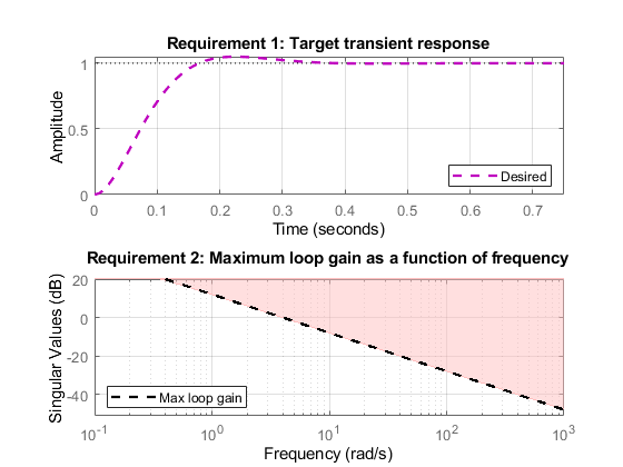
Create a tunable PID control and design according to the following goals:
- Reference tracking: percent overshoot < 5% and settling time of 0.3 sec.
- Maximum loop gain: imposes a maximum gain constraint on the complementary sensitivity function
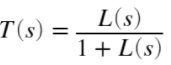 of the system. In this case, we want a 0 dB gain at 4 rad/s with -20 dB/dec afterwards.
% create tunable PID control
C = tunablePID('C','pid');
% fix set-point and filter constant parameters
C.Tf.Value = 1/500;
C.Tf.Free = false;
% add analysis point at control input
AP = AnalysisPoint('u');
% Find Y(s)/R(s) closed-loop transfer function (i.e. reference to output)
CL0 = feedback(GxbIc*AP*C,1);
CL0.InputName = 'r';
CL0.OutputName = 'y';
% Nominal tunable closed-loop system
CL0_Nom = feedback(GxbIc.NominalValue*AP*C,1);
CL0_Nom.InputName = 'r';
CL0_Nom.OutputName = 'y';
%
% Ball setpoint reference tracking goal
Rtrack = TuningGoal.Transient('r','y',tfdes,'step');
% Max loop gain: 0 dB gain at 4 rad/s
Rmaxgain = TuningGoal.MaxLoopGain('u',4,1);
% View goals
viewGoal([Rtrack, Rmaxgain]);
The tuning is performed using the Control System Tuner using both the nominal and uncertain plants. Robust tuning is when tuning is applied to the plant with the uncertain parameters. The performances of the nominal and robust controllers are then compared both when simulated and run with the actual hardware.
% Setup tuner options
opt_ST = systuneOptions('RandomStart',2);
% NOMINAL PLANT TUNING
[CLNom,fSoftNom] = systune(CL0_Nom,[Rtrack, Rmaxgain],opt_ST);
Final: Soft = 24.7, Hard = -Inf, Iterations = 57
Final: Soft = 24.7, Hard = -Inf, Iterations = 73
Final: Soft = 24.7, Hard = -Inf, Iterations = 58
showTunable(CLNom);
C =
             1            s
  Kp + Ki * --- + Kd * --------
             s          Tf*s+1


  with Kp = -156, Ki = -956, Kd = -2.4, Tf = 0.002

Name: C
Continuous-time PIDF controller in parallel form.
CtunedNom = getBlockValue(CLNom,'C');
% UNCERTAIN/ROBUST PLANT TUNING
rng(0), [CL,fSoft] = systune(CL0,[Rtrack, Rmaxgain],opt_ST);
Nominal tuning:
Design 1: Soft = 24.7, Hard = -Inf
Design 2: Soft = 24.7, Hard = -Inf
Design 3: Soft = 24.7, Hard = -Inf

Robust tuning of Design 2:
Soft: [24.7,210], Hard: [-Inf,-Inf], Iterations = 73
Soft: [27.9,30.3], Hard: [-Inf,-Inf], Iterations = 27
Soft: [29.2,29.2], Hard: [-Inf,-Inf], Iterations = 27
Final: Soft = 29.2, Hard = -Inf, Iterations = 127

Robust tuning of Design 3:
Soft: [24.7,210], Hard: [-Inf,-Inf], Iterations = 58
Soft: [27.9,30.3], Hard: [-Inf,-Inf], Iterations = 27
Soft: [29.2,29.2], Hard: [-Inf,-Inf], Iterations = 27
Final: Soft = 29.2, Hard = -Inf, Iterations = 112

Robust tuning of Design 1:
Soft: [24.7,210], Hard: [-Inf,-Inf], Iterations = 57
Soft: [27.9,30.3], Hard: [-Inf,-Inf], Iterations = 27
Soft: [29.2,29.2], Hard: [-Inf,-Inf], Iterations = 27
Final: Soft = 29.2, Hard = -Inf, Iterations = 111
% [CL,fSoft] = systune(CL0,[Rtrack, Rmaxgain]);
showTunable(CL);

C =

             1            s
  Kp + Ki * --- + Kd * --------
             s          Tf*s+1

  with Kp = -179, Ki = -484, Kd = -2.41, Tf = 0.002

Name: C
Continuous-time PIDF controller in parallel form.
Ctuned = getBlockValue(CL,'C');
Robust and Nominal Control Simulation Results
The step responses of the nominal and robust controllers are first simulated in MATLAB. Because the robust controller uses the uncertain model, it shows the responses for different values of the electromagnet force constant.
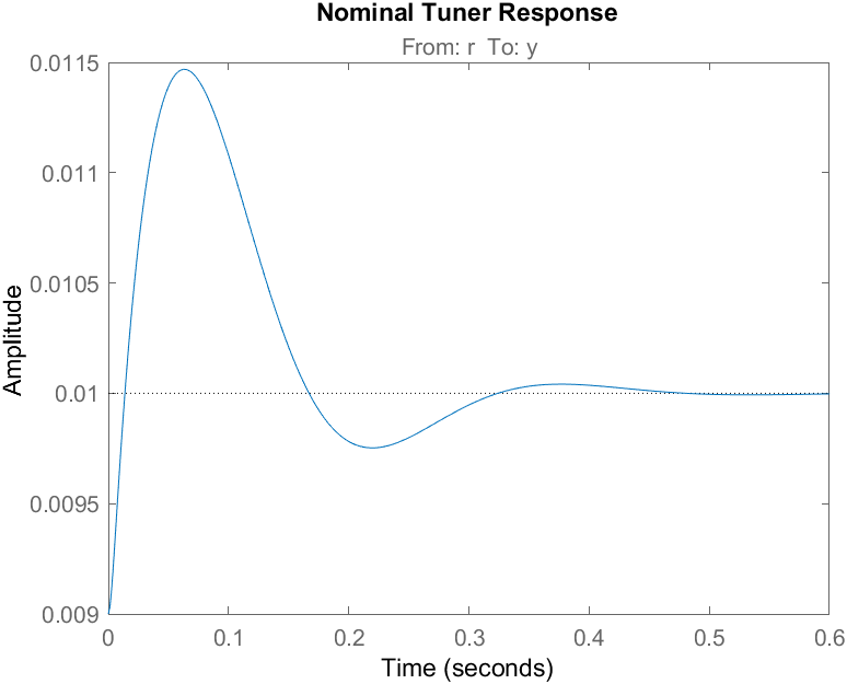
The nominal control is based on the nominal model with a fixed electromagnet constant and is used a reference point. We also simulate the worst-case scenario of the robust controller, which is when the ball is close to the magnet.
% Simulate 1 mm step about operating point
opt = stepDataOptions('InputOffset',9e-3,'StepAmplitude',1e-3);
title("Robust Tuner Response");
step(CL,opt);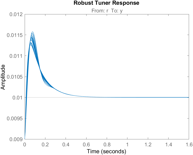
% Simulate closed-loop control with nominal parameters
title("Nominal Tuner Response");
step(CLNom,opt);
% Find worst-case case and frequency
[wcg,wcu]=wcgain(CL);
% Simulated worst-case closed-loop rddesponse
CL_wc = usubs(CL,wcu);
step(CL_wc,opt);
title('Worst-Case Response');
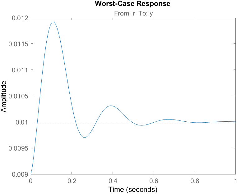
As shown, the overshoot increases and more oscillations occur as the ball approaches the magnet. Given this, we can use robust tuning techniques to design PID gains that will yield a better response over a larger operating range.
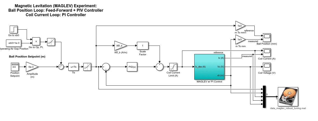
The MATLAB simulations use the linearized model. A more representative simulation is performed in a Simulink model that includes:
-
- Nonlinear model of the Maglev system.
- Linear model of the electromagnet with a PI current control.
- Electromagnet current range: 0 to 3 A
- Ball position range: 0 to 14 mm
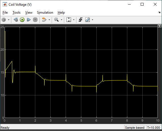
- Amplifier output voltage range: -24V to 24V.
- Variable electromagnetic force constant based on experimental data shown earlier.
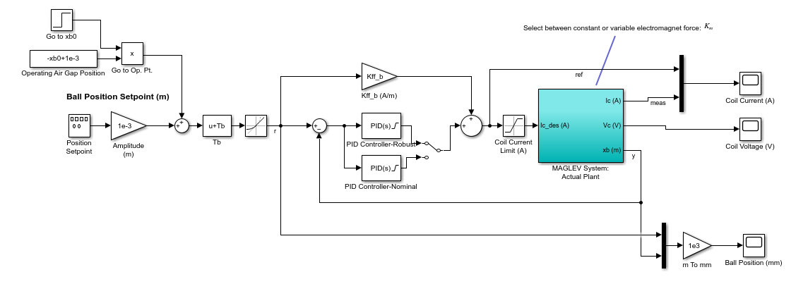
Here the results are more in-line with the tracking overshoot and settling time specifications defined earlier.
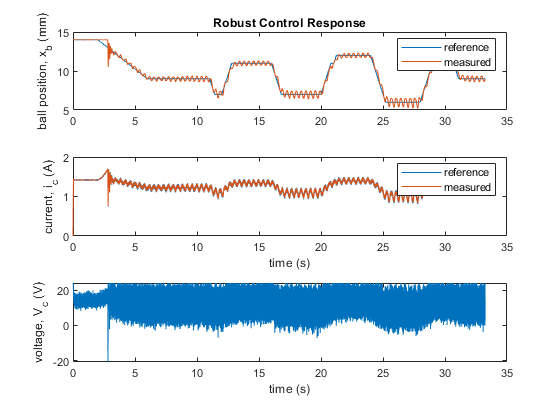
Robust Control Implementation Results
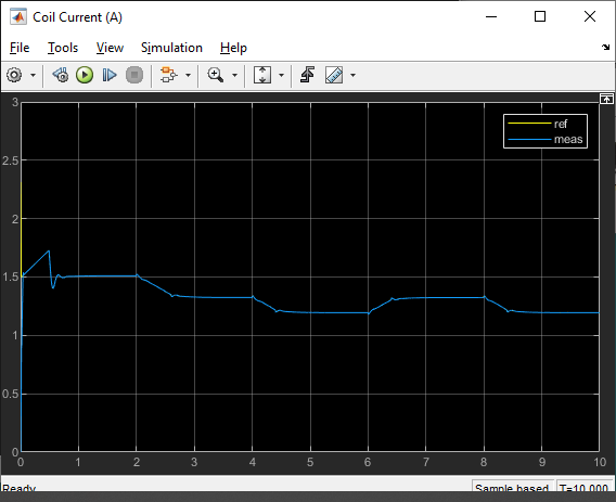
The PID gains generated from the tuner with the uncertain plant are run using the actual Maglev hardware with Simulink and the Quanser QUARC Real-Time Control Software.
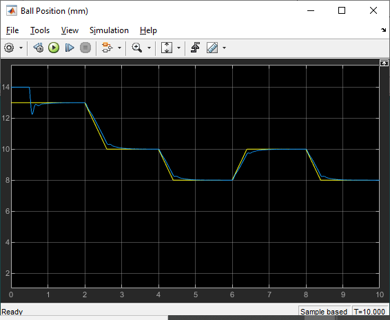
The ball is first stabilized at an air gap of 9 mm. A +/- 2 mm square wave ball position reference command is then applied in the first cycle and then increased to +/- 3 mm.
Here is a video of the robust control in action:
Nominal Control Implementation Results
The PID gains generated using the model based on a fixed electromagnet constant is then ran on the system. Similar as in the test above, the ball is stabilized at 9 mm and a square wave command with an amplitude of +/- 1 mm in the first cycle, +/- 2 mm in the second cycle, and +/- 3 mm is the last is applied.
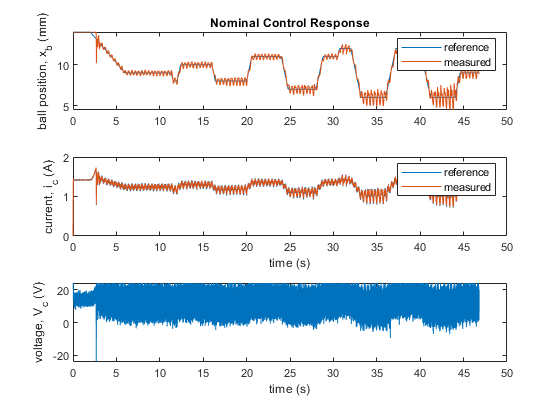
When comparing the reference tracking response of each control, the ball position is more oscillatory in the nominal control as the ball goes closer to the magnet (i.e., smaller air gap). This is in line with what we had noticed in the worst-case simulation response. The robust control handles this operational range more effectively.
Final Remarks
There are many other, more advanced robust control methods, e.g., H-Infinity synthesis, that could be implemented here. Hopefully this is a good introduction to the MathWorks® Robust Control Toolbox™ and how it can be used get a better response in challenging control system.
Resources
Robust Control Toolbox™ MathWorks® page:
https://www.mathworks.com/products/robust.html?s_tid=srchtitle_robust%20control%20tuning_1
Robust Control Turning MathWorks® help page:
https://www.mathworks.com/help/robust/robust-tuning.html
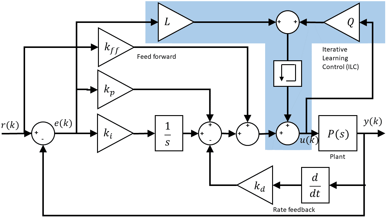
Using Iterative Learning Control (ILC) on the Maglev:
https://www.quanser.com/blog/iterative-learning-control-for-magnetic-levitation/
Magnetic Levitation System for Teaching “Intermediate” Control:
https://www.quanser.com/blog/nonlinear-system-for-intermediate-control/