
In introductory control system courses, the analysis is typically done in the S-domain using transfer functions, and the advanced control courses introduce students to the state-space modeling and state-feedback control techniques. But quite often, instructors are caught in the mid-range situations, where they want to expose students to advanced control systems without requiring them to use state-space techniques. In my previous blog post from the “intermediate control” series, I suggested the Ball and Beam system as a great way to introduce intermediate-level control concepts. Today, I’d like to highlight another system that fits well in between the “classic” and “modern” control: a Magnetic Levitation plant.
Nonlinear Electro-Mechanical System for Hands-on Lab Experimentation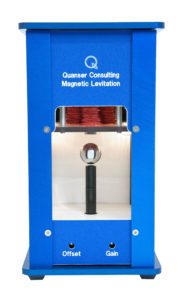
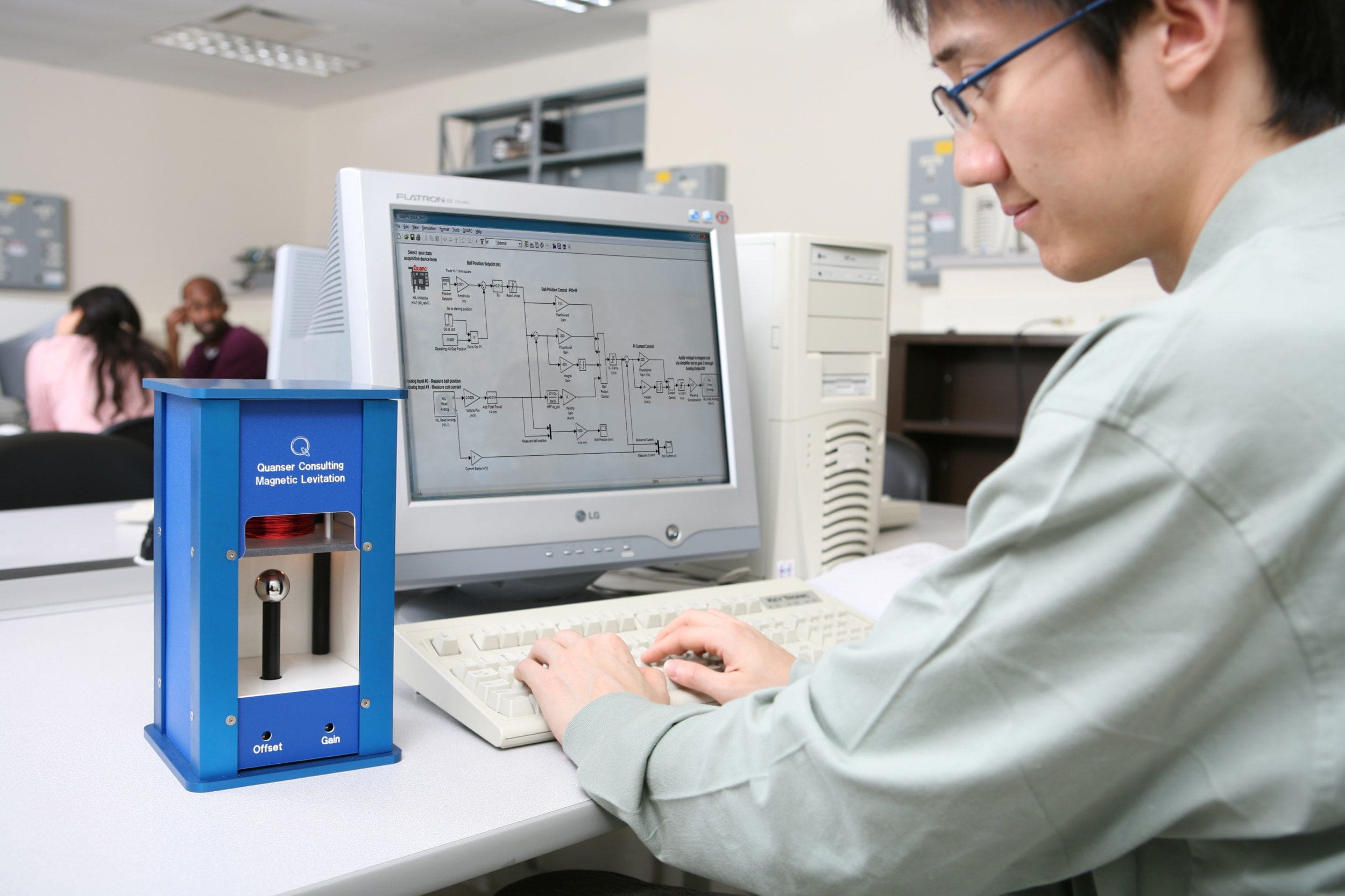
The Quanser Magnetic Levitation is a single degree of freedom system with an overhead electromagnet that generates an attractive force on a metal ball placed on a post. The position of the ball is measured using a photo-sensitive sensor embedded inside the post. The system also includes a current sensor to measure the current inside the electromagnet’s coil.
The force acting on the ball increases very fast as the ball approaches the magnet (i.e., as the air gap becomes smaller). Further, the current response in the electromagnet is slow due to its large inductance. Thus, there are actually two subsystems – ball/electromagnet dynamics and electromagnet voltage/current dynamics. One way to address this is by using a cascading controller: a current control for the magnet, and an outer ball position controller.
Modeling and Control Design
The dynamics of the Magnetic Levitation system is shown in the figure below.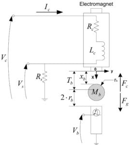
As mentioned earlier, the attractive force that is exerted on the steel ball from a standard electromagnet is nonlinear:

The force is proportional to the current squared, and the size of the air gap squared. As the ball approaches the face of the electromagnet and the air gap decreases, the force increases substantially. The electromagnet constant, Km, is based on the properties of the electromagnet material, dimensions, coil winding, and so on. While this is modeled as a constant, this parameter actually varies over the operation time as the inductance in the electromagnet increases and depending on the air gap between the ball and the magnet.
The nonlinear equation of motion of the ball with respect to the commanded current can be described by the expression:

As shown, the system is nonlinear due to the two square terms on the current and air gap.
As mentioned earlier, because of the large inductance in the electromagnet core, the actuator has its own dynamics and can be modeled with Kirchhoff’s Law to get the electrical equations:
![]()
where Rc is the coil resistance, Lc is the coil inductance, Ic is the coil current, vc(t) is the applied coil voltage, and Rs is the current sense resistance. From this, we can obtain a first-order transfer function of the circuit:
![]()
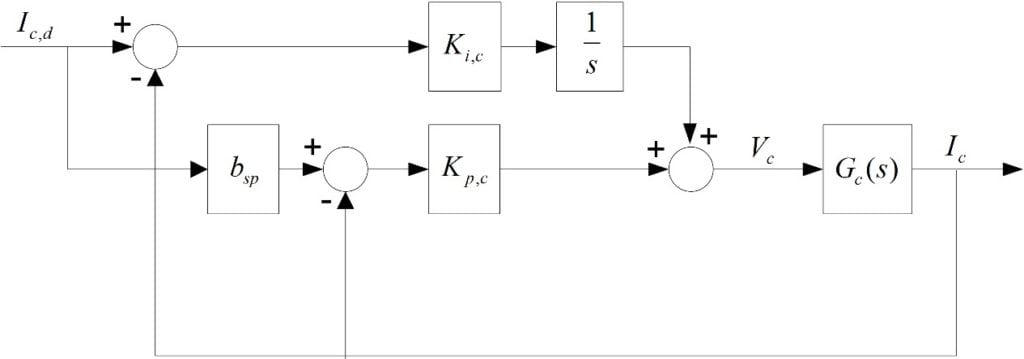
The time constant of a core with a large inductance can be, for instance, around 0.035 sec. A time constant this large would be detrimental to the control of the ball because the desired current in the coil required to stabilize the ball takes too long to reach that point. As a result, a control such as Proportional-Integral compensator shown in the figure below is needed to regulate the voltage of the electromagnet for the desired current to match the measured one.
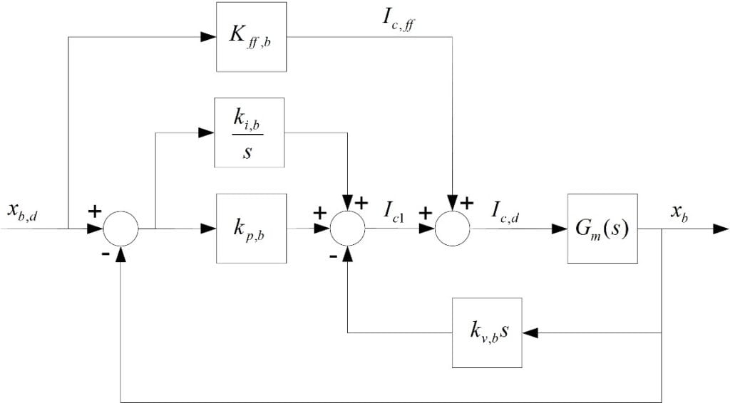
The ball position can be done by using a PID-based compensator shown in the figure below. The nonlinear equation of motion (EOM) is first linearized about its operating point to obtain the linear EOM and its corresponding transfer function. Then we can design a PID control according to certain time-domain performance criteria, such as peak time and overshoot. Incorporating a feed-forward loop that includes a gain based on the known model improves the response time to ball position commands and minimizes the effort of the integral term.
Takeaway
Magnetic Levitation is a great system to introduce new control challenges. Students need to learn about linearization to design a PID controller, implement cascade control loops to compensate for slow actuator dynamics, and add feed-forward control to improve the response time.
Want more?
To further improve the control response, you can design a more advanced controller such as gain scheduling. Because the magnetic force constant, Km, actually changes depending on the air gap, varying the control gains based the current ball position as the system is in operation results in more precise and robust control. An example of a gain scheduler is available on our QuanserShare site: search for Magnetic Levitation – Gain Scheduling.
In the next post of the intermediate control system series, we’ll look at a Coupled Tanks system. This nonlinear system illustrates challenges of the liquid level control, a common issue in many industrial processes.