
The challenge for many professors and instructors teaching a control systems course is to find practical, easy-to-use, and well-documented hands-on devices that could help make the theoretical concepts more concrete. In the introductory control system courses, the analysis is typically done in the S-domain using Transfer Functions. These are sometimes referred to as ‘classic control systems‘ concepts. The second or third control courses, often called ‘modern control systems,’ introduce students to the state-space modeling and state-feedback control techniques. The state-space approach is great, for example, when working with more advanced MIMO systems.
Circuits and DC motors are often used to teach classic modeling and control concepts, while systems like inverted pendulums and other MIMO systems are used for more advanced modern control system concepts. But what about the mid-range situations, where the instructor wants students to learn and develop advanced control system without requiring them to use state-space techniques? In this blog series, I would like to highlight some of the systems that are great for an intermediate-difficulty control systems level.
Ball and Beam: a bridge between DC Motor Control and advanced MIMO systems
 The Ball and Beam is a very classic control experiment that is a perfect bridge or middle-point challenge between DC motor control and more advanced MIMO systems, like an inverted pendulum. It can address the need for more complex dynamics/control challenge without requiring students to know about modern control concepts such as state-space.
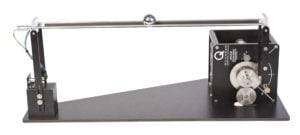
The Quanser Ball and Beam is one of the add-on modules for the Rotary Servo Base Unit (SRV02) system. The objective is to stabilize the ball along the beam to the desired setpoint. The elevation of the beam is controlled using the rotary servo system, the angle of the servo is measured using an incremental optical encoder, and the ball position is measured using a linear potentiometer sensor.
Modeling
This section shows how to model the Ball and Beam system by, first, deriving its nonlinear equation of motion, linearizing it about an operating point, and obtaining the corresponding Transfer Function.
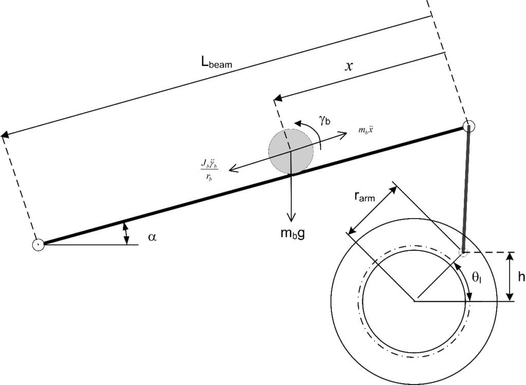
The free-body diagram of the rotary Ball and Beam system is represented in the following figure:
Assuming friction is negligible, the equation of motion of the ball is
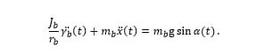
When translating the rotational motion of the ball, γb, into a linear motion, the equation becomes:
![]()
Note that this system is nonlinear because of the sine function. The rotary servo is used to control the angle of the beam, α(t). The relationship between the beam angle and the angle of the servo load gear is
![]()
where rarm is the distance between the center of the load gear and where the beam arm is attached, and Lbeam is the length of the beam, as depicted in the Free body diagram of the ball on a beam figure above. Substituting this to the equation of motion above gives the expression
![]()
Solve the expression for the ball acceleration to get
![]()
Given that the moment of inertia of the ball is
![]()
the equation for the ball acceleration can be simplified to
![]()
Interestingly enough, the motion of the ball on the beam is not affected by mass or dimensions of the ball itself, but rather the architecture of the ball and beam system.
To obtain the linear equation of motion, linearize the nonlinear EOM about the beam being horizontal Ɵ(t) = 0:
![]()
where
![]()
The control input is the servo motor voltage. We need to develop a position control for the servo in order to control the angle of the system (i.e., to stabilize the ball). The servo dynamics between the motor voltage applied and the angle of the servo can be modeled by the transfer function:
![]()
Control Design
For the control design, we can have two cascading control systems: inner servo position control and an outer ball position control.
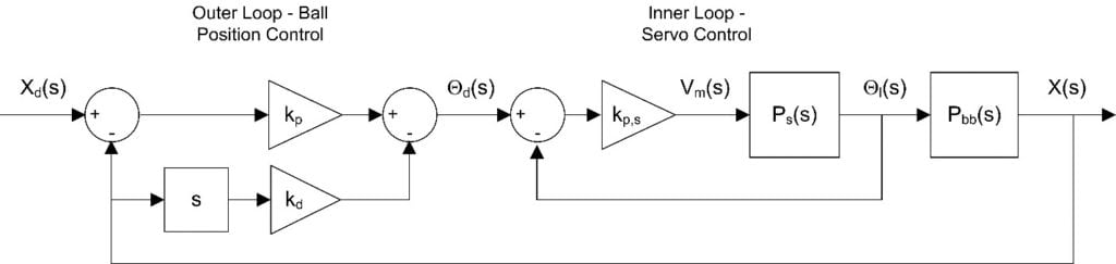
Assuming the servo position control has very good tracking control, we can assume the desired and measured angle of the servo are the same, i.e., Ɵ(t) = Ɵd(t). The servo position command now becomes the control input of the outer ball position control, and we can then design a PD control for the ball position as follows:
![]()
The closed-loop equation is second-order
![]()
The outer controller computes the desired angle for the rotary servo in order to move the ball to the desired position. The desired servo angle, Ɵd(t), is fed into the inner servo control which applies the DC motor voltage needed to move the servo angle to that position.
Takeaway
The Ball and Beam is a more complex system that requires isolating two different subsystems and using more advanced control techniques, such as cascading control loops. But the control design can all be done using classic control techniques: PID and transfer functions. It doesn’t require the student to know state-space modeling and state-feedback control, which may not have been introduced yet.
Want more?
You can challenge your students to try to balance the ball along the beam manually, using the mouse, as described in this video:
You can download the controller from our QuanserShare site (and feel free to share any controller that you developed!): search for Ball and Beam Mouse Controller.
In the next post of the intermediate control system series, we’ll look at a Magnetic Levitation. Also nonlinear, the problem of levitating a ball using an electromagnet poses new challenges for the controls engineer.