
Model Predictive Control (MPC) has been around for a long time but has found new applications in tasks such lane following for Self-Driving vehicles. Likewise, although traditionally used to control plants with slow dynamics in the process control industry, it can also be used for higher speed motion control applications like balancing an inverted pendulum. Here, we show how to develop an MPC balance control for the Qube-Servo 3 system using The MathWorks® Model Predictive Control Toolbox™ for Simulink®. MPC is implemented on the QLabs Virtual Qube-Servo 3 system and the Quanser Qube-Servo 3 hardware using the QUARC Real-Time Control software.
Using Model Predictive Control for the Qube-Servo 3
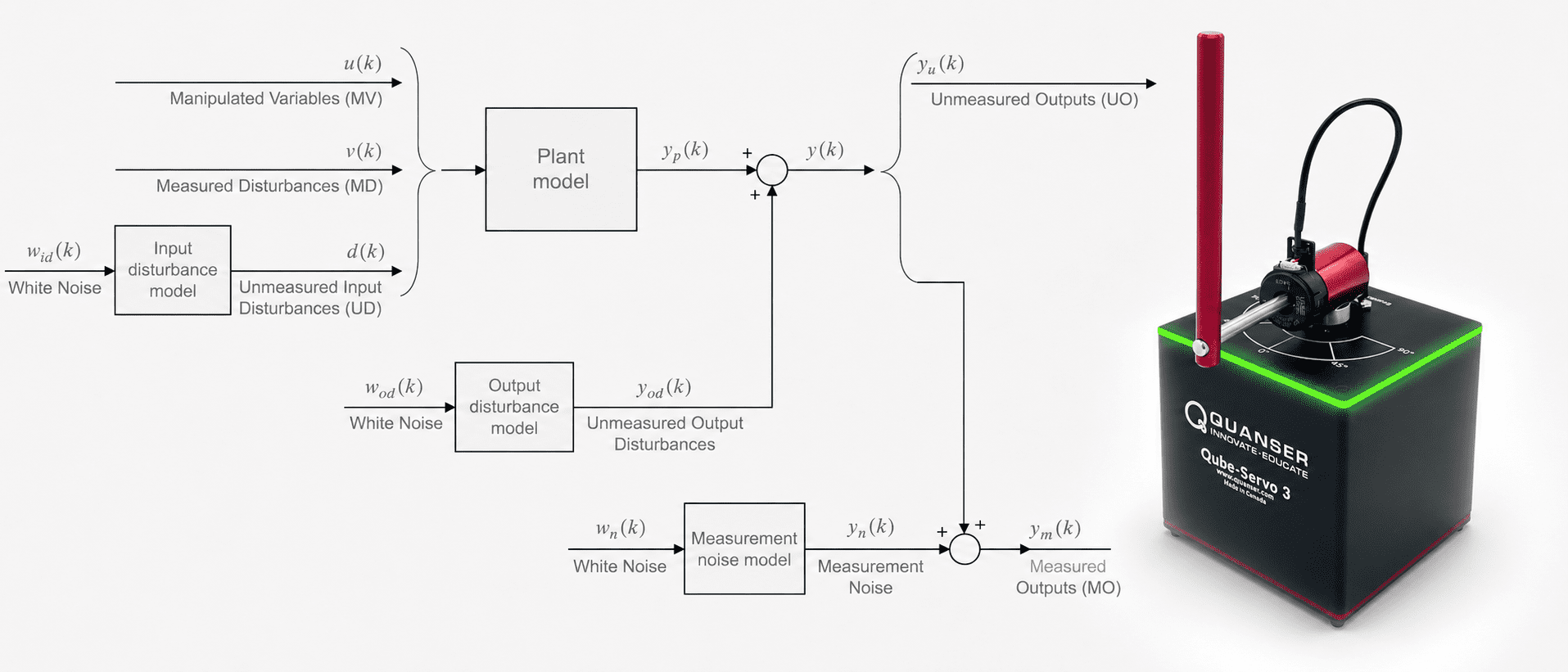
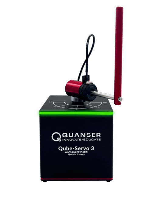
The Quanser Qube-Servo 3, shown below, can be configured as a DC motor or an inverted pendulum plant for teaching and research in control systems. In the supplied courseware, we go through the design of a state-feedback control to balance the pendulum, e.g., using Linear Quadratic Regular (LQR). State-feedback control follows a model-based design approach and performs well. But it doesn’t consider unmodeled uncertainties and disturbances, such as the effect of the encoder cable. If the model does not accurately represent the system, then the controller may not perform adequately and as expected.
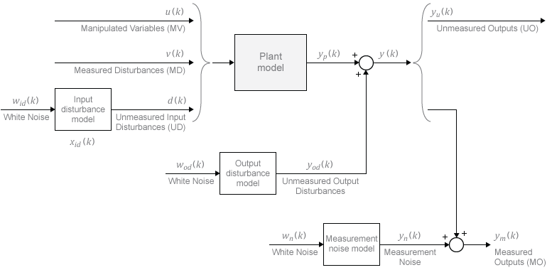
The MathWorks® Model Predictive Control toolbox makes it easy to design and implement MPC controllers. The MPC design starts with defining the various input and output signals and their limits. Figure 2 illustrates the plant model signals used in the MPC controller. You still need to have a representative model, but because of its adaptive nature, less control design is required and it can compensate more for effects such as parameter uncertainties and disturbances.
Qube-Servo 3 MPC Design
The sample time, prediction horizon, and control horizon are the key parameters when creating an MPC. The prediction and control horizon need to be adjusted according to the sample time required for the application. See Choose Sample Time and Horizons for design guidelines.
Balancing the Qube-Servo 3 inverted pendulum typically needs at least 200 Hz for good performance. In the standard state-feedback control, a sample rate of 500 Hz is used to achieve better control. In MPC, using a higher sampling rate requires higher prediction time and that is more computationally intensive. The design guideline of T ~ NpTs where T is the desired closed-loop time and Ts is the sampling interval, can give a good starting point. If we want a closed-loop response of 0.25 sec, then we need a prediction horizon of approximately Np = 125.
This can be used as a starting point and then tuned in the closed-loop simulation to get the desired response and ensure it’s not too computationally intensive.
Ts = 0.002; % sampling interval (s)
Np = 150; % prediction horizon
Nc = 2; % control horizon
qube_ip_mpc = mpc(rotpen_ss, Ts, Np, Nc); % mpc control
The Qube-Servo 3 control input, i.e., the manipulator variable (MV), is the motor voltage and the recommended maximum output of the power amplifier is ±10V. Measured Outputs (MO) are the rotary arm and inverted pendulum. When in balance mode, the rotary arm typically does not surpass ±60 deg. This is assuming we keep commands within this range, and it does not go unstable. Balance control is only active when the pendulum is within ±10 deg within the upright vertical position. Given this we can set the following min/max limits and scale factors on the manipulated variable (MV) and measured outputs (MO):
% min/max control input (V)
u_max = 10;
u_min = -10;

% min/max rotary arm angle (rad)
theta_min = -60*pi/180;
theta_max = 60*pi/180;

% min/max inverted pendulum angle (rad)
alpha_min = -10*pi/180;
alpha_max = 10*pi/180;
Specify scale factors for inputs and outputs
qube_ip_mpc.ManipulatedVariables.ScaleFactor = u_max-u_min;
qube_ip_mpc.OutputVariables(1).ScaleFactor = theta_max-theta_min;
qube_ip_mpc.OutputVariables(2).ScaleFactor = alpha_max-alpha_min;
Set min/max of manipulated variables (i.e., motor input).
qube_ip_mpc.ManipulatedVariables.Min = u_min;
qube_ip_mpc.ManipulatedVariables.Max = u_max;
The weights on the manipulator variables and output variables are typically what can fine tune the performance of the control. It’s an iterative process done through closed-loop simulation. After a few iterations, we finalized using the following weights:
qube_ip_mpc.Weights.ManipulatedVariables = 0;
qube_ip_mpc.Weights.ManipulatedVariablesRate = 0.1;
qube_ip_mpc.Weights.OutputVariables = [10 5];
The OutputVariables weight was adjusted from [1 0]. The first weight affects the rotary arm, and it was increased to 10 to have better setpoint tracking. The second weight is associated with the pendulum and was increased to minimize the deflection.
Note: In this example, adding min/max limits to the Output Variables made the MPC creation process very slow. For this application, it was best to start with fewer limits and testing the simulation.
Model Predictive Control – Running the Simulation
The Quanser Qube-Servo 3 system comes supplied with full documentation, including courseware for the student and instructor, as well as the Simulink® models and MATLAB scripts used to design and simulate an LQR-based state-feedback balance control. The Model Predictive Control designed above is implemented using the MPC Controller block from the Model Predictive Control Toolbox™. The supplied state-feedback based Simulink® model was modified to include the MPC Controller block as shown below.
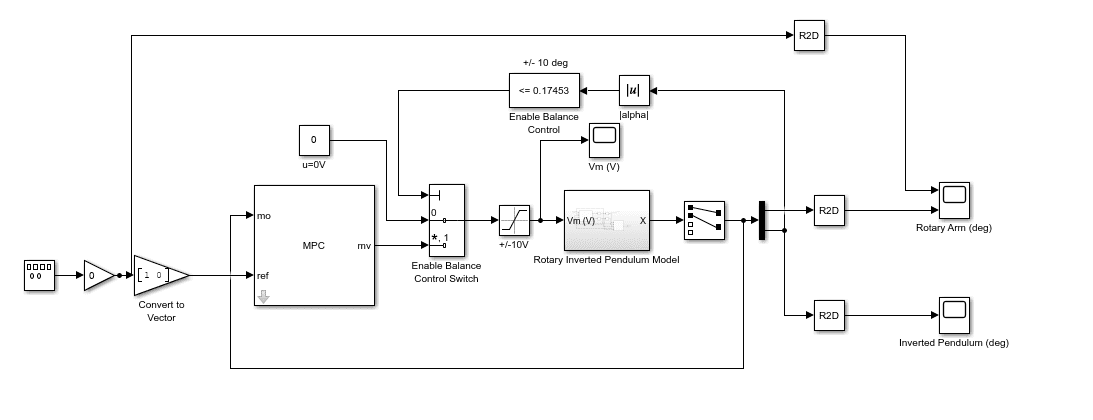
Figure 3: Simulink model to simulate Qube-Servo 3 Inverted Pendulum MPC balance control.
The Simulink diagram includes a nonlinear model of the Qube-Servo 3 inverted pendulum to get a more representative response of the actual system. The response of the rotary arm and pendulum when the pendulum starts at 9 deg from the upright balance position is shown in the Rotary Arm (deg) and Inverted Pendulum (deg) scopes. The voltage applied to the motor is shown in the Vm (V) scope.
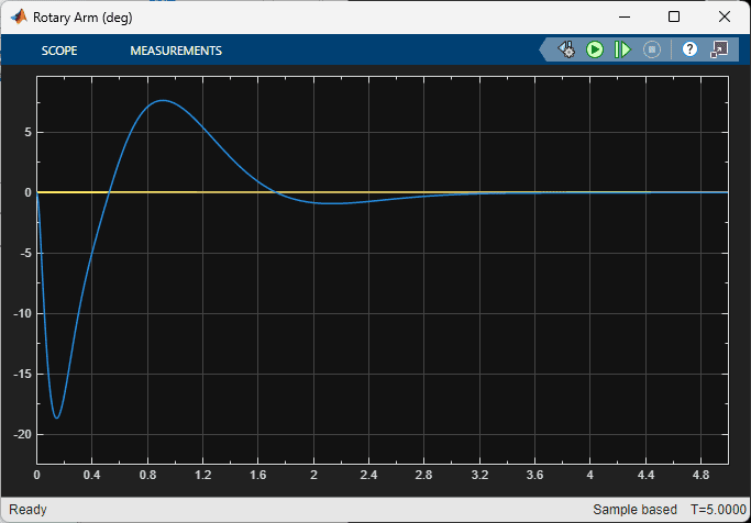
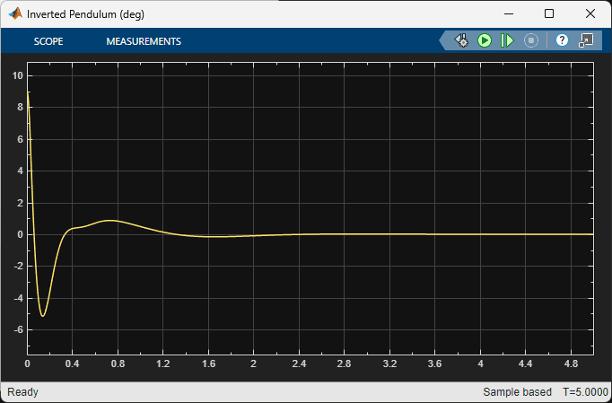
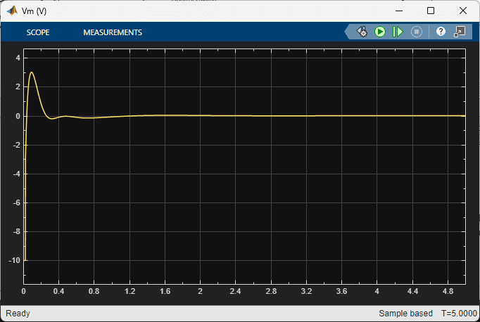
Figure 4: MPC pendulum balance control simulation response.
Model Predictive Control – Running it on the Virtual System
The QLabs Virtual Qube-Servo 3 system includes a high-fidelity nonlinear dynamic model of the Qube-Servo 3. This includes friction, hardware limits, sensors noise, and other characteristics that standard models don’t account for.
As done in the simulation, we implement the MPC designed above on the Virtual Experiment using the MPC Controller block from the Model Predictive Control Toolbox™. However, an Enabled Subsystem block is used to activate the MPC Controller only when the pendulum is about the +/- 10 deg upright position. This ensures the built-in Kalman filter estimates the states of the system accurately. Otherwise, the estimates take too long to give an accurate estimate, and the pendulum cannot be balanced (i.e., goes unstable).
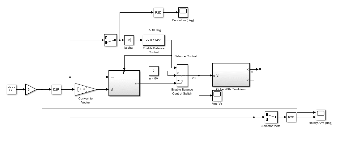
Figure 5: Simulink model to run Qube-Servo 3 Inverted Pendulum MPC balance control on Virtual Qube-Servo 3.
The scopes below show the response when the pendulum is brought up from the downward position, and the balance control is engaged on the virtual Qube-Servo 3.
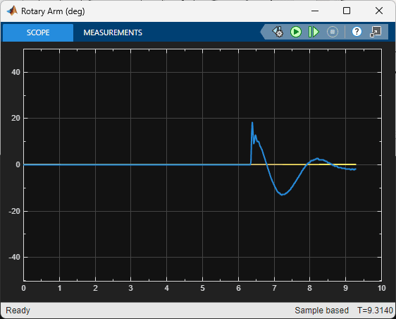
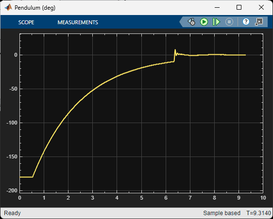
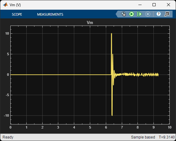
Figure 6: Response of MPC inverted pendulum balance control using virtual Qube-Servo 3.
The response is slightly different from the simulation results obtained. With the virtual system, we see the response includes some high-frequency components, e.g., this could be attributed to encoder quantization, which is incorporated in the virtual system.
Model Predictive Control – Running it on the Hardware
The Simulink model below implements the MPC controller designed on the Quanser Qube-Servo 3 hardware. The MPC control designed is implemented using the MPC Controller block from the Model Predictive Control Toolbox™, similarly as in the virtual plant. The hardware interface and deployment is performed with the QUARC Real-Time Control software.
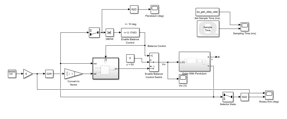
Figure 7: Simulink model to implement Inverted Pendulum MPC balance control on Qube-Servo 3 hardware.
A sample response when MPC is run with QUARC on the physical hardware is shown in the response below. It is similar to the virtual twin.
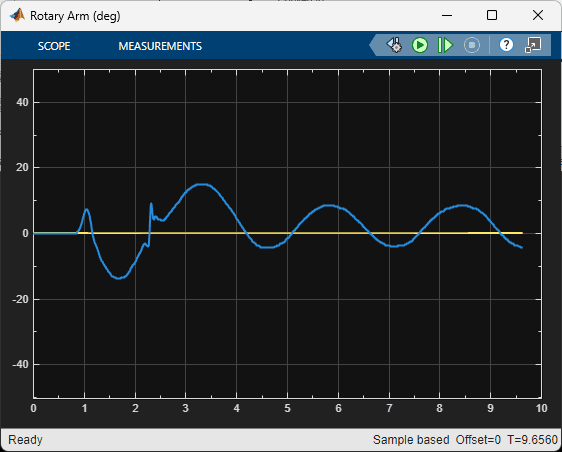
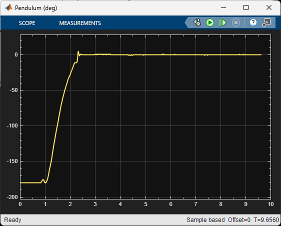
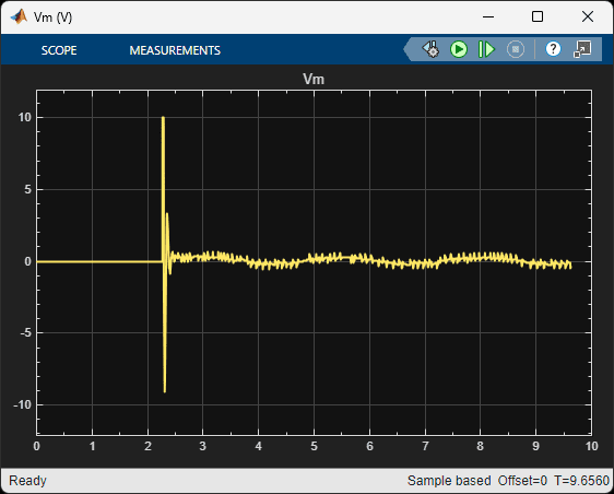
Figure 8: Response of MPC inverted pendulum balance control on Qube-Servo 3 hardware.
Future Work
Model Predictive Control (MPC) can be used on a variety of systems. There are also different types of MPC controllers. For the Qube-Servo 3 Inverted Pendulum, we designed and implemented the standard implicit MPC control. In the future, we plan on exploring other types of MPC that are available in the Model Predictive Control Toolbox™ for Simulink®. One application that has been investigated is using Nonlinear MPC to perform the pendulum swing-up. Nonlinear MPC allows us to use the nonlinear model to perform such tasks.
Resources
Please visit the MathWorks website for more information on the Model Predictive Control Toolbox:
- MathWorks® Model Predictive Control Toolbox™ product page: https://www.mathworks.com/products/model-predictive-control.html
- Choosing Sample Time and Horizons: https://www.mathworks.com/help/mpc/ug/choosing-sample-time-and-horizons.html
- 3 Ways to Speed Up Model Predictive Controllers: https://www.mathworks.com/content/dam/mathworks/white-paper/3-ways-to-speed-up-model-predictive-controllers.pdf