
I spent a fair bit of time working in the oil and gas industry where you come across many sophisticated control systems. Given the complexity and interconnectivity of those systems, it is often operationally and financially undesirable or even unsafe to shut down a part of the system for tuning purposes. As a result, online control tuning techniques are commonly used. So, when I recently came across an autotuning block in Simulink®, I had to give it a try with our Virtual QUBE-Servo 2 to see how well it works tuning the gains of a PI (proportional-integral) speed controller on-the-fly.
What is Controller Tuning?
Controller tuning is the process of adjusting the parameters of the controller to achieve a desired dynamic response. For example, in the case of a proportional-integral-derivative (PID) controller, tuning the controller means adjusting kp, ki, and kd gains such that the system being controlled produces a desired overshoot or rise time. There are numerous ways to tune a PID controller, from manual and heuristic methods (which require no or little mathematics) such as the Ziegler–Nichols method, to pole placement design where the gains around found based the model and desired specifications. Make sure to check out the MATLAB Tech Talk that my friend Brian Douglas has made on controller tuning.
What is Simulink’s Closed-Loop PID Autotuner Block?
The Closed-Loop PID Autotuner block is part of the Simulink Control Design™ toolbox and it lets you tune a PID controller in real-time starting with a set of initial controller gains that results in a stable loop. The advantages of autotuning methods such as this – and why it’s used in industry so much – is the system remains under closed-loop control with the initial PID gains and the gains are tuned without needing a model of the plant. It is a very practical technique. The block lets you tune your controller to achieve a specified bandwidth and phase margin without a parametric plant model.
How Does it Work?
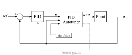
The diagram below shows how the PID Autotuner block could be integrated into a PID controller. The block works by performing a frequency-response estimation experiment by injecting test signals into your plant. The test signals are sinusoids at the frequencies [1/10, 1/3, 1, 3, 10]ωc, where ωc is the specified target bandwidth for tuning. You can start the autotuning process by applying a non-negative value to the start/stop port, or applying a zero or negative value to stop the tuning process.
The autotuner finds PID gains based on the estimated frequency response and the desired bandwidth and phase margin. Once the autotuning process has stopped, the tuned PID gains can be applied to the PID controller block to validate the closed-loop performance in real-time. Keep in mind that until the autotuning process begins, the block relays the PID control signal, u, directly to the plant input, u +Δu.
Example using QLabs Virtual QUBE-Servo 2
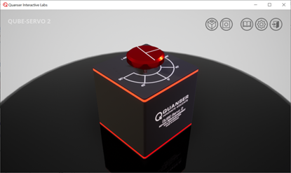
Since I did not have a physical QUBE-Servo 2 with me, I decided to test out the Closed-Loop PID Autotuner block on the QLabs Virtual QUBE-Servo 2.
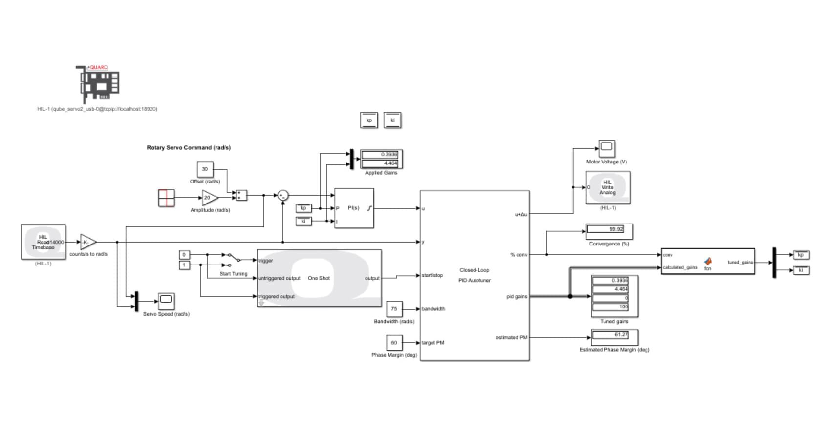
Below is the controller that I used as part of my test. If you already have QLabs and MATLAB/Simulink and would like to try it out, you can download the controller from here. If you don’t have QLabs, sign up for a free trial!
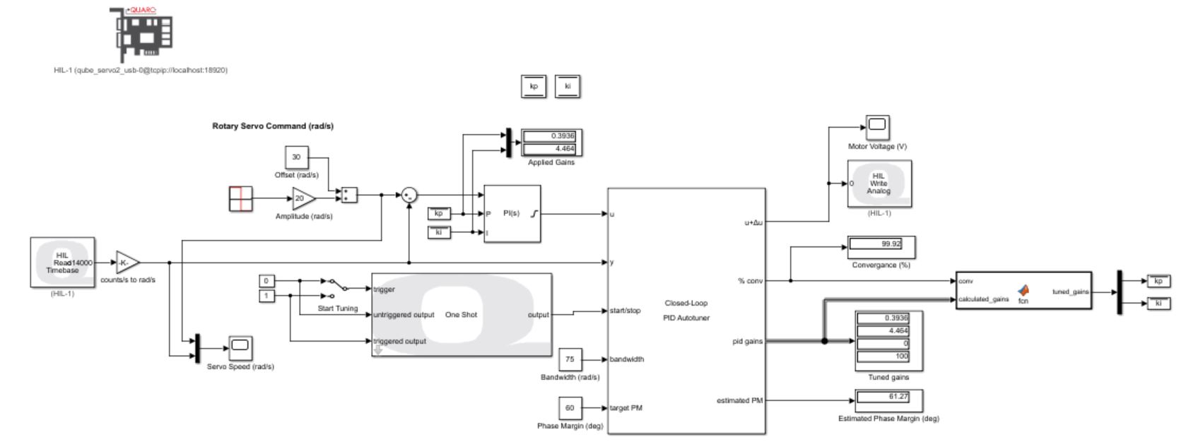
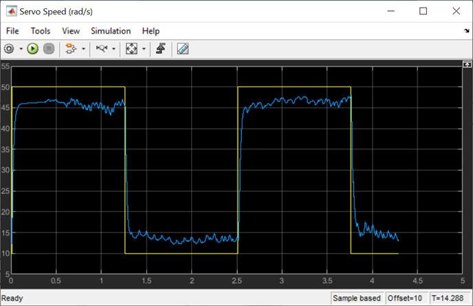
The Simulink model implements a PI speed controller. A square wave with a frequency of 0.4 Hz is commanded to the virtual QUBE to alternate the speed of the load shaft between 10 rad/s and 50 rad/s. I started off by using kp and ki values of 0.2 and 0.1, respectively. These gains were not tested prior, but I was fairly confident that they would not result in an unstable system. I configured the Autotuner block with my desired bandwidth and phase margin values of 75 rad/s and 60 deg respectively. With the Start Tuning manual switch set to 0 (effectively bypassing the Autotuner block), I ran my model. Below is the untuned response that I observed.
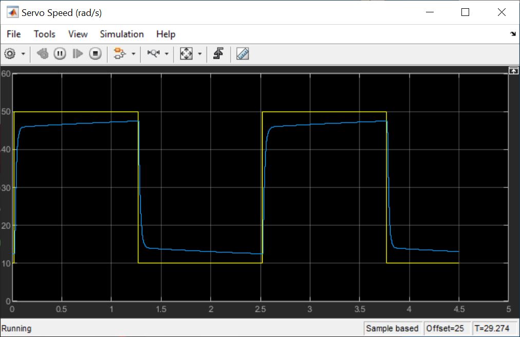
After toggling the Start Tuning manual switch block, the Autotuner blocks started to interject the test signals to my virtual plant. The sine amplitude of the test signals was set to 0.1, but you can change that value to see how it affects the results. Below is the response of the virtual QUBE while being subjected to the test signals.
I used the QUARC™ One Shot block to produce a pulse signal that would run the Autotuner block for 4 seconds. During this time, my model monitored the %conv output of the Autotuner block. Once the value converged to 98%, tuning was considered complete, and the Simulink diagram displayed the tuned gains as well as the estimated phase margin. I also implemented some logic in my model to transfer the tuned gains generated by the autotuning block to the PI controller. This means that I did not have to stop my model to apply the tuned gains to the plant.
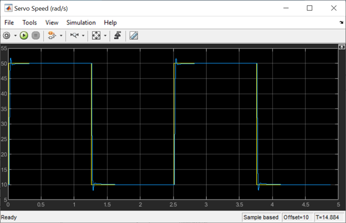
Below is the system response upon completion of the autotuning process and applying the new controller gains. And you can see a far better response compared to the untuned controller that I started off with. The resulting estimated phase margin was 58 deg (very close to the desired 60 deg) and the calculated tuned gains were kp = 0.38 and ki = 2.68.
There you have it! With the Closed-Loop PID Autotuner block I managed to conduct an online tuning of the speed controller for my virtual plant and apply the tuned gains on the fly with no downtime. Why not download my model and sign up for a free QLabs trial to give it a try yourself? Or better yet, try running the model on a physical QUBE-Servo 2 if you have one!
References
- How PID Autotuning works: https://www.mathworks.com/help/slcontrol/ug/how-pid-autotuning-works.html
- When to use PID autotuning: https://www.mathworks.com/help/slcontrol/ug/when-to-use-pid-autotuning.html
- Closed-Loop PID Autotuner: https://www.mathworks.com/help/slcontrol/ug/closedlooppidautotuner.html
- PID Autotuning in Real-Time: https://www.mathworks.com/help/slcontrol/ug/pid-autotuning-in-real-time.html