
In a previous blog, I discussed how to create 2D occupancy grid maps for navigation purposes using 2D Lidar scans. In this blog, however, I’d like to highlight some of the advantages of creating 3D maps, as opposed to 2D maps, using a process called Real-Time Appearance-Based Mapping (RTAB-MAP). I’ll also show how I implemented this technique on a Quanser QCar in ROS.
What is RTAB-MAP?
RTAB-MAP is a graph-based SLAM approach using RGBD cameras, stereo cameras, or a 3D Lidar. These sensors serve as an incremental appearance-based loop closure detector. The process uses a bag-of-words method to determine whether each newly acquired frame of image (or Lidar scan) came from a previous location or a new location. A graph optimizer is then applied to minimize the errors based on the frame. Throughout the process, a memory management scheme is applied to limit the number of locations used for the loop closure detection and graph optimization – this is to ensure acceptable real-time performance when dealing with a large-scale environment.
Why is RTAB-MAP important?
One of the advantages of using a 3D map over a 2D one is the three-dimensional visual presentation of objects. From a 2D map, we only know the distance information at the elevation of where the Lidar is located, which typically is located at the top of the autonomous car. As a result, the distance information at ground level or anywhere in between the elevation of the Lidar and ground is unknown, which is why autonomous navigation hardly utilizes 2D occupancy maps. This is one of the reasons our QCar adds 4 CSI wide-angle cameras and an RGBD camera at the top to ensure an inclusive collection of visual information.
Consider an autonomous vehicle that operates in an underground coal mine. The space that it operates within typically has narrow tunnels with sharp turns in all directions. The vehicle needs enough information about what’s in front of it so it can plan its speed and trajectory accordingly. In this example, GPS navigation is not possible since the vehicle is underground, and odometry data solely based on wheels is not accurate since there will be slippage under the wheels. Therefore, RTAB-MAP becomes very useful, as long as the vehicle is equipped with an RGBD camera pointing forward to collect 3D information. Based on the algorithm that RTAB uses, the vehicle will be able to calculate visual odometry data that can be fused with wheel odometry data.
QCar Implementation
I decided to implement this using the RGBD camera on the QCar by doing a 3D SLAM using the rtabmap_ros package. The implementation is fairly straightforward:
- Launching RGBD camera to collect depth data,
- Drive the QCar using a gamepad and,
- Plot the 3D map and the car’s trajectory.
To launch the RGBD camera, you only need to run the ROS package for the Intel Realsense camera:
roslaunch realsense2_camera rs_camera.launch align_depth:=true
The last argument is to align the depth camera information with the colour camera to make sure the depth information is aligned with every pixel in the colour camera frame. One of the benefits of using ROS is the strong ROS community which provides many ready-to-go packages that lets you quickly get your applications up and running. Once you’ve launched the RGBD camera, the next step is to drive the QCar using a gamepad. The tools I’m using are Simulink and our powerful real-time control software QUARC. Our engineers have spent tremendous time on creating different autonomous driving applications using those tools. If you want to see how exactly we implement manual drive in Simulink, please go to this website to download it.
The last step is to visualize the data using the following commands:
roslaunch rtabmap_ros rtabmap.launch
rtabmap_args:=”–delete_db_on_start”
depth_topic:=/camera/aligned_depth_to_color/image_raw
rgb_topic:=/camera/color/image_raw
camera_info_topic:=/camera/color/camera_info
approx_sync:=false
rtabmapviz:=false
rviz:=true
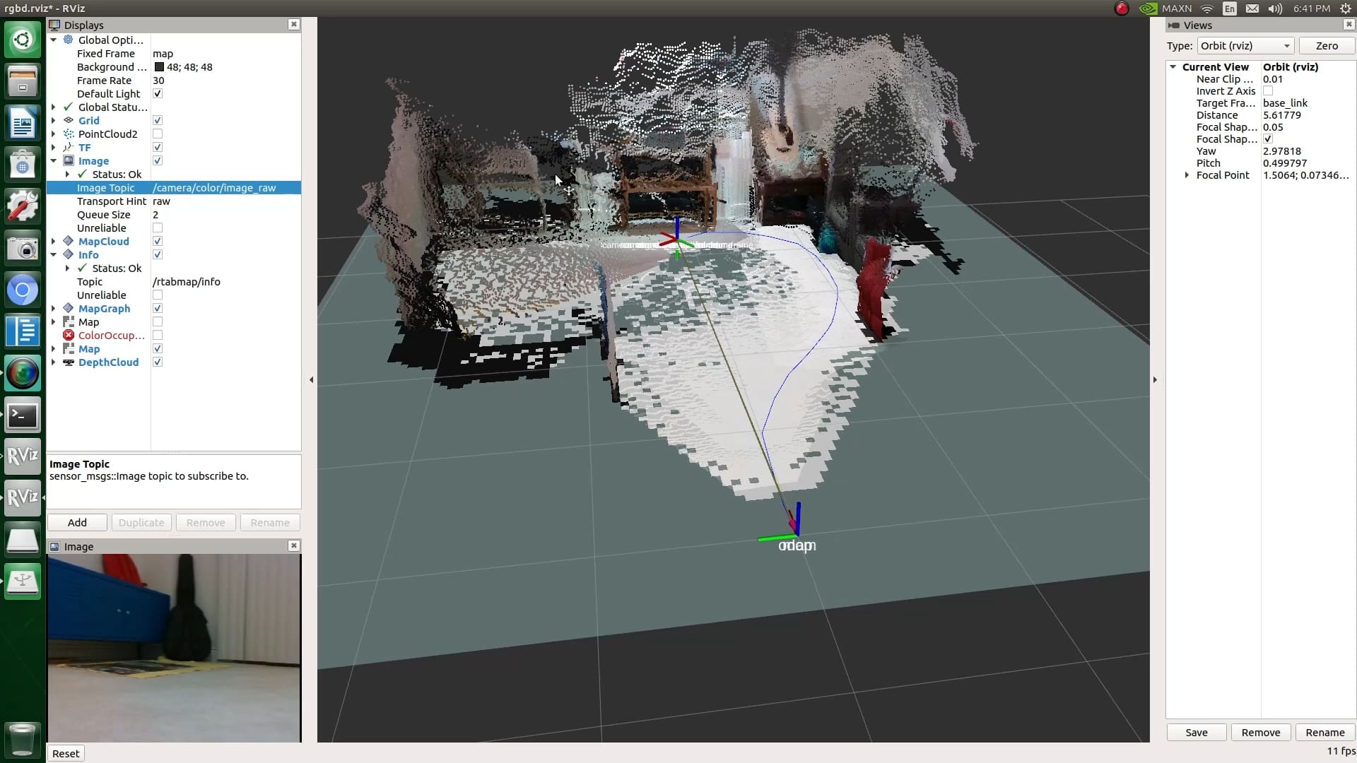
The arguments followed by the main command are to inform the ratbmap algorithm to subscribe to the correct topics coming from the RGBD camera and to open the visualization tool. A 3D map from the RGBD camera is shown in the space. After calculating the distance information, it will also plot a 2D occupancy grid map on the floor.
In the video below, as I drive the QCar around, the map is updated based on the detection of loop closure and a trajectory is calculated from the visual odometry. The algorithm is quite robust, even when the QCar does a sharp turn as it approaches the end of the room. When the QCar comes back, you can see that the 3D visualization map has no shift which indicates that the 3D map and the localization data that it generates are accurate.
What can be improved?
Given the nature of the RGBD camera, the default refresh rate is set to 60 Hz. Therefore, the optical flow sensor will lose its confidence if the frame is moving too quickly. Moreover, the lighting condition in the environment must be sufficient, otherwise, the algorithm will have difficulty detecting whether the frame is updated and may not compare it with the previous frame. Fortunately, we can fuse the odometry data with our Lidar technology. Since I’m a ROS user, my next implementation to improve the performance is to fuse the pose data coming from hector slam with the odometry data. Given that Lidar is not constrained with the lighting condition and we’ve previously tested the performance of our Lidar, I can trust the pose data coming from it.
Self-driving technology is now booming. A single RGBD camera can lead to many applications in different disciplines. Imagine what could be possible to have all the sensors combined? I hope this blog highlighted one of the numerous applications that can be implemented on a QCar. If you have questions about this blog or QCars in general, drop a comment below or contact us via email at info@quanser.com