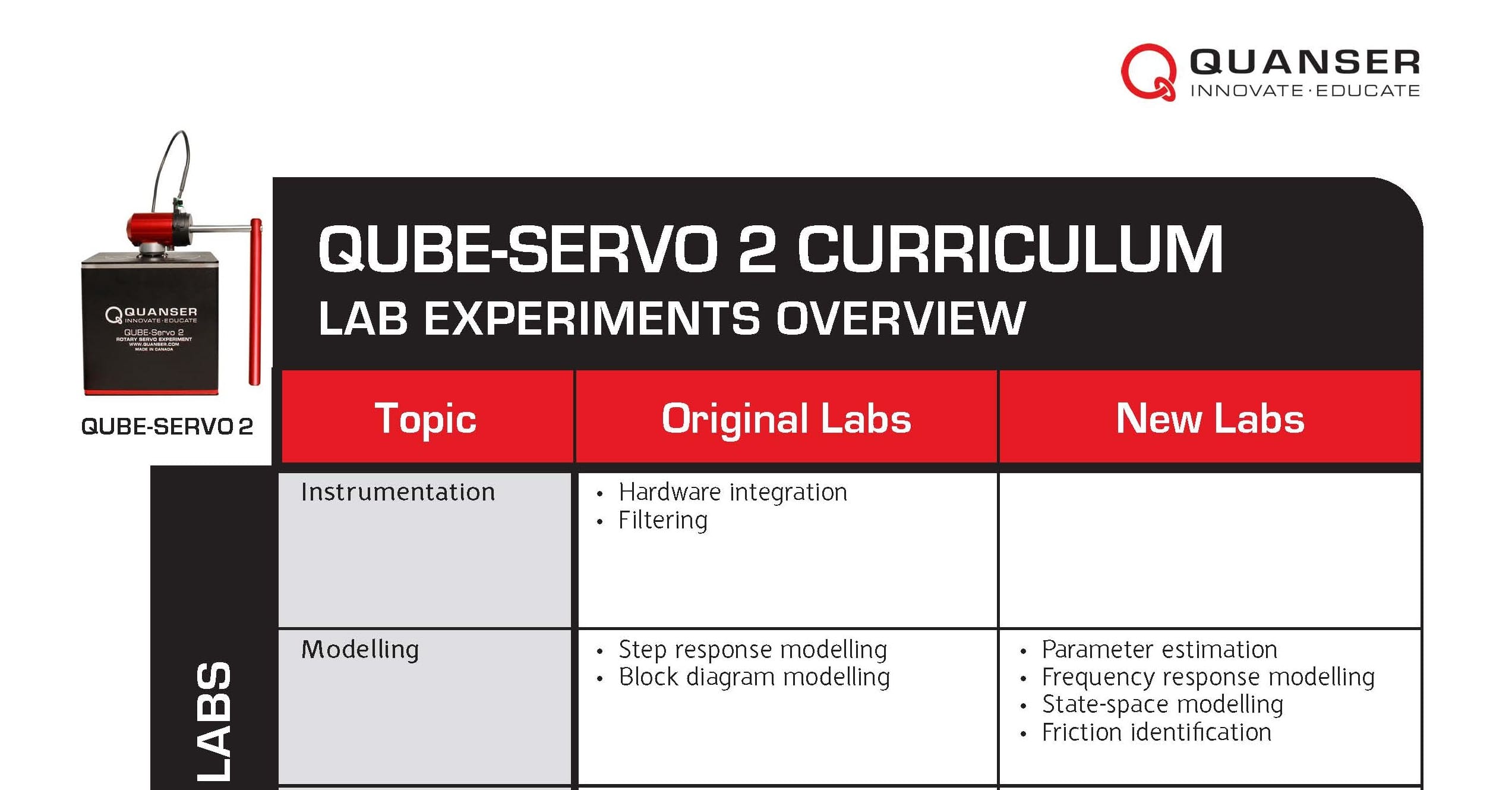

In my previous blog post, I walked you through the new and expanded curriculum for our popular QUBE-Servo 2 system. I also highlighted the institutions and educators whose input and feedback helped us bring in new topics and develop new labs. In this post, I want to delve deeper into the areas of instrumentation and modelling, where we added four new lab experiments: parameter estimation, frequency response, state-space modelling, and friction identification.
 Why Instrumentation?
Instrumentation is a science of measurement and control of process variables. It’s a large field that is related to controls and industrial automation. Common tasks include interfacing hardware and software through a data-acquisition (DAQ) device and sensor calibration. Both of these tasks are necessary before implementing a control system.
Overview of QUBE-Servo 2 Instrumentation Labs
In the QUBE-Servo 2 curriculum, you can find these Instrumentation labs:
| Lab | Description |
| Hardware Interfacing | Learn how to interface to the servo motor and encoder using Simulink and QUARC. |
| Filtering | Derive velocity measurement from the encoder sensor. |
Hardware Integration
The Hardware Integration lab is typically the first lab students go through. It sets the foundation – this is where students learn about the QUBE-Servo 2 hardware and how to use the software tools such as Matlab/Simulink and QUARC real-time control software to interface to the motor and sensors of the system.
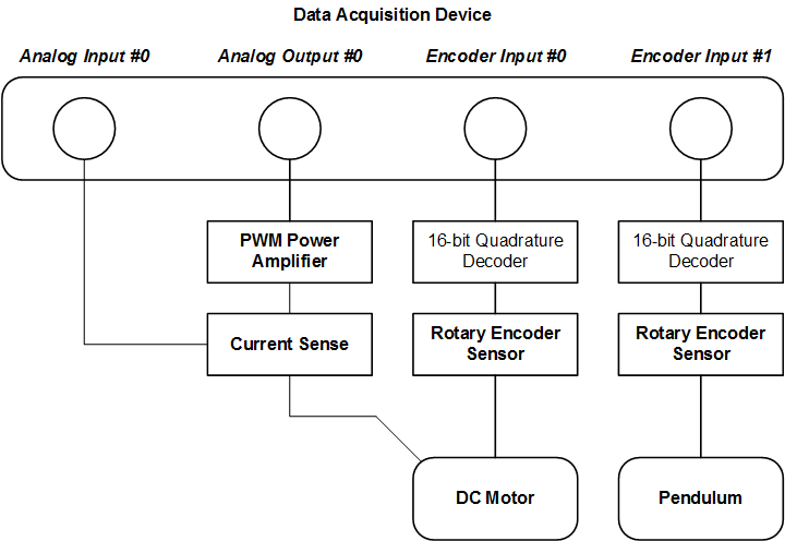
The interface between DAQ and QUBE-Servo 2 hardware
Filtering
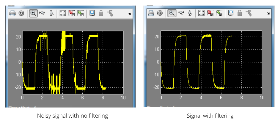
Filtering is widely used in many different industries, often when dealing with analog sensors that have noise and are used in feedback control. In the case of the QUBE-Servo 2 Filtering lab, we show how filtering is needed when the velocity is derived from the encoder-based position measurement. The figures below compare the unfiltered signal with the filtered version. Which one would you like to use in a control system?
Why Modelling?
Obtaining a model of the system – like a transfer function or state-space representation – is typically done so you can use it to design a control system. The model can then be used to run simulations and validate that the system requirements are met. That increases the chances that the controller will work on the actual system and reduces the number of design iterations.
Overview of QUBE-Servo 2 Modelling labs
The modelling labs – both old and new – are summarized in the table below.
| Lab | Description |
| Step response modelling | Find the model of the system experimentally by applying an input step. |
| Block diagram modelling | Model the servo from first-principles using a block diagram and the known system parameters. |
| Parameter Estimation | Measure the resistance and back-emf constant of the system and find the corresponding first-order transfer function model. |
| Frequency Response Modelling | Derive the model of the system using a sine wave at varying frequencies. Also includes phase delay analysis |
| State-Space Modelling | Derive the linear state-space representation of the system and validate it by running it in parallel with the hardware. |
| Friction Identification | Measure the Coulomb and Viscous friction of the motor. |
Experimental Modelling
Step response and frequency response are two experimental modelling techniques that are sometimes called “black box” methods. It means they don’t require system parameters or full dynamic models of the system. They are commonly used for systems with unknown dynamics, or when the model is too difficult to derive from first-principles. The model is found by examining the relationship between the input signal and the output response. For a DC motor system like QUBE-Servo 2, we use these methods to identify the parameters of a first-order transfer function that represents the position or speed of the motor with respect to the voltage applied.
In the Step Response Modeling lab, the model is derived by examining the output motor speed response when a step voltage is applied, as illustrated in the figure below. It is also known as the “bump test” method.
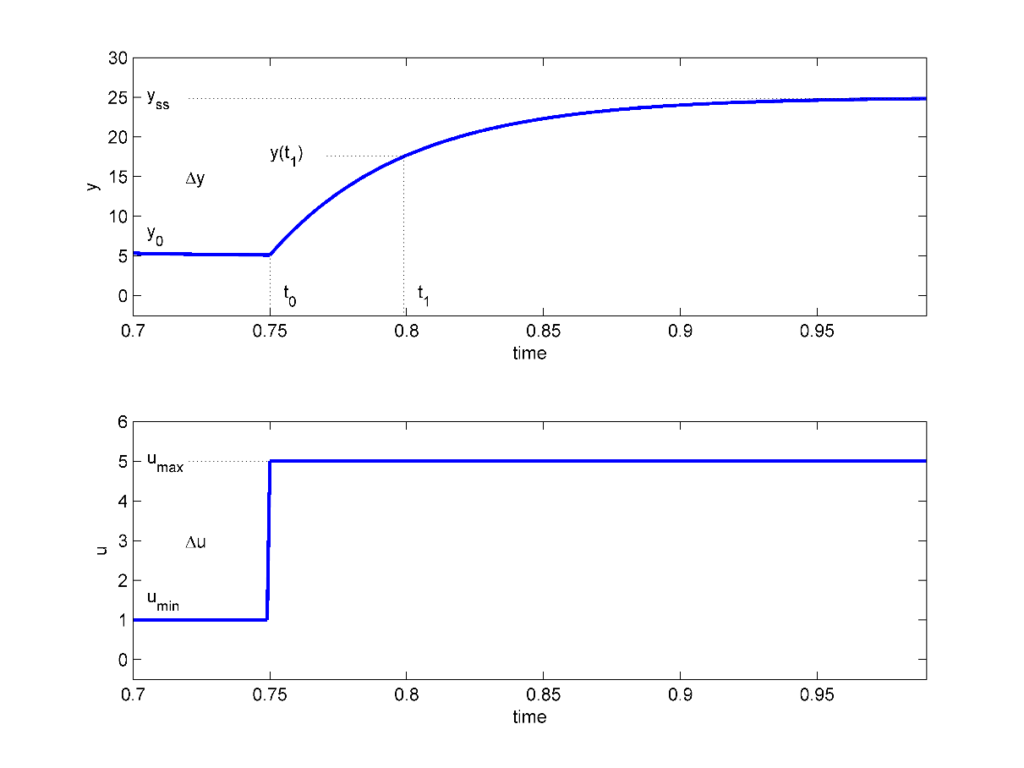
Step response modelling
Frequency response is a classic method that has been used for many years. In this case, a sine wave of varying frequencies is applied to the system. The corresponding sinusoidal output response is then used to build a Bode plot. From that, the transfer function model parameters can be identified. The plot below shows an example response when applying an input voltage signal, u, and measuring the output motor speed response, y.
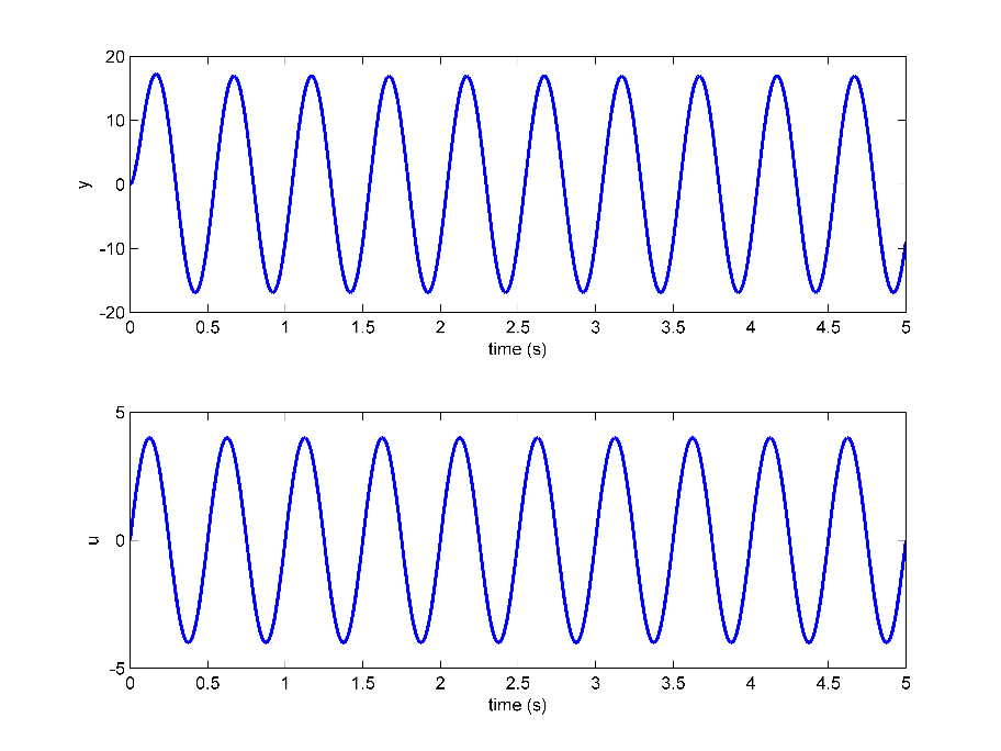
Frequency response
Pros and Cons of Experimental Modelling
“Black box” modelling methods are nice because they don’t take long to perform (compared to deriving it from first-principles) and can also yield accurate models. Their main drawback, however, is that they cannot be used on unstable systems or systems with limits. For instance, you cannot use a step response to model a cart on a 1 m track because the cart may go to one of the end stops.
Theoretical Modeling
When the dynamics of the system are known, as is the case with QUBE-Servo 2, we can derive its equations of motion (EOMs) from first-principles using a free-body diagram similar to this one:
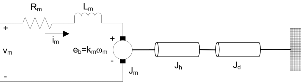
Model of QUBE-Servo2
In the Block Diagram Modelling lab, the QUBE-Servo 2 model is implemented in a Simulink diagram using standard Simulink blocks, e.g., Integrator and Sum blocks. An example of a block diagram is shown below. Once the block diagram is complete, students verify if the model is correct by running it in parallel with the hardware, using QUARC real-time software. This is known as a “model validation.” It’s an important part of the modelling process and is performed in all of the QUBE-Servo 2 modelling labs.
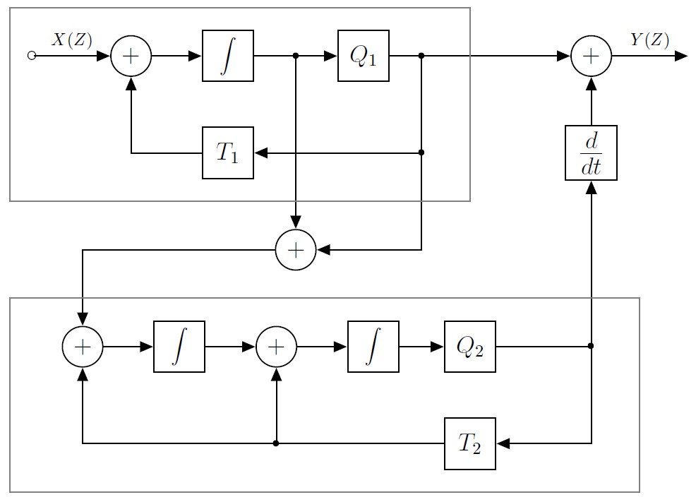
Block diagrams can be used to model systems with known dynamics, like the QUBE-Servo 2.
Pros and Cons of Theoretical Modelling
Modelling a system from first-principles using a block diagram requires an in-depth knowledge of how the components interact with each other. You also need to know the system parameters (e.g., motor shaft inertia). The dynamics of the system must also be known in order to model the system from first-principles. Further, theoretical modelling may be difficult to perform on complex systems and may neglect certain aspects that are captured in, for instance, experimental modelling methods.
Parameter Estimation through Experimental Tests
In other cases, we may have the model, but the system parameters for that model are either not available or inaccurate. In the Parameter Estimation lab, the equations derived from first-principles are used to get the equations needed to evaluate the motor resistance and back-emf parameters. However, for these equations, the motor resistance and back-emf parameters of the DC motor have to be found experimentally.
Pros and Cons of Parameter Estimation
The Parameter Estimation method combines the traits of theoretical and experimental modelling. There is still an emphasis on “knowing your system” in order to derive the model, but you don’t need to know all the system parameters. Because the parameters are found experimentally, without using the manufacturer’s specifications that vary slightly between units, you can obtain a more accurate model. The main disadvantage, similarly to the “black box” modelling methods, is that parameter estimation is only feasible on certain systems (non-volatile systems, for one). It also requires all the necessary sensors. For example, this lab could not be performed on the previous version of the system, QUBE-Servo 1, because it did not have a current sensor.
Model Representation
Transfer functions are commonly used to model many systems and are also used in most of the QUBE-Servo 2 labs. The other common representation used is state-space. State-space modelling is applied in higher-complexity, Multiple Input Multiple Output (MIMO) systems like robot manipulator arms.
The newly added State-space Modelling lab is a great way to introduce state-space representation using a simpler system and to put it into practice by validating whether your model represents the system accurately or not. This can then lead to state-feedback control, which sets the foundation to design advanced control for more complex systems, e.g., balancing an unstable pendulum.
Nonlinear and Unmodeled Dynamics
 Linear models are used to characterizing systems in many applications. However, physical systems, data-acquisition devices, and so on, all have nonlinear elements that are neglected in the modelling process.
In the Friction Identification experiment, we highlight the most commonly neglected elements in models: Coulomb friction and Viscous friction.
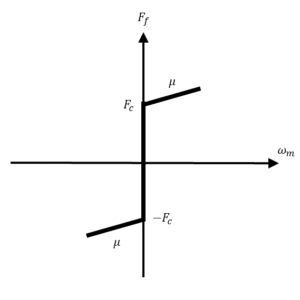
A sample friction model
Pros and Cons of Friction Identification
Most systems have friction. Knowing how friction affects the system response is a huge value-add because that’s usually what students first notice when going from simulation to implementing their controller on the actual device: the response doesn’t match up. But including friction in the model is not always necessary. In fact, typically, friction is treated as being “negligible” because most applications use linear controllers. Linear controller design is based on a linear model, which cannot include nonlinear elements such as Coulomb friction. In addition, there are fairly simple ways to compensate for friction after the initial design, e.g., tuning the control gains, adding integral control.
I hope this post provides you with a good overview of the instrumentation and modelling labs included in the curriculum accompanying the QUBE-Servo 2 system. I will talk about the other concepts we cover in one of my future articles.