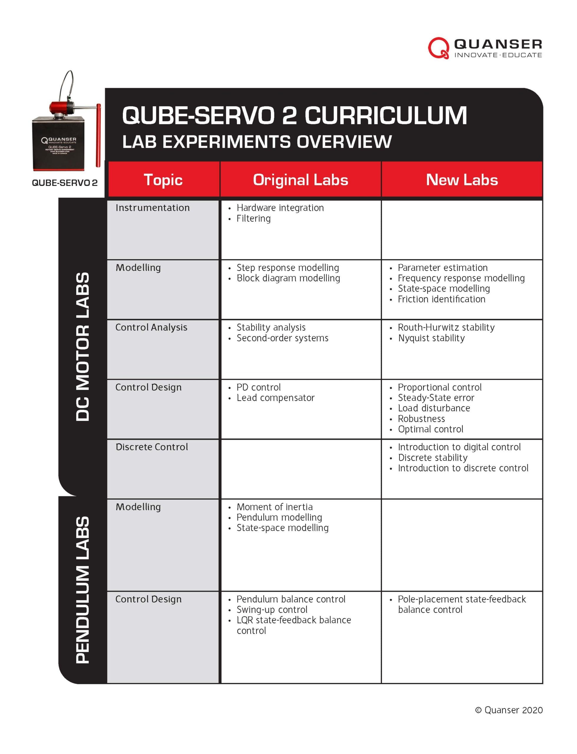

A few weeks ago, we released a major update of the curriculum developed for one of our most popular products, QUBE-Servo 2. Adding new and expanding already covered concepts, we more than doubled the number of lab experiments in the lab material. In my previous blog post, I highlighted the Instrumentation and Modelling labs included in the courseware, today I will shift my focus on System Analysis and Control Design labs.
Why perform system analysis?
System analysis is a natural precursor to control design. Looking at the properties of the system, e.g., whether or not it is stable, how much overshoot it has, and so on can help you select the best type of control to get a certain desired response.
Overview of QUBE-Servo 2 System Analysis labs
The system analysis labs – both old and new – are summarized here:
| Lab | Description |
| Stability analysis | Assess the stability of the DC motor system based on the Bound Input Bounded Out (BIBO) response and pole locations. |
| Second-order systems | Learn about second-order system parameters, i.e., natural frequency and damping ratio, and see how they affect the system response. |
| Routh-Hurwitz Stability | Use the Routh-Hurwitz method to assess the stability of the DC motor system and design a control gain. See how the Routh-Hurwitz assessment translates in the actual hardware response. |
| Nyquist Stability | Assess the stability margins of the system using the Nyquist diagram and then find them experimentally on the actual servo. |
Stability Analysis
Two of the most fundamental ways of assessing the stability of a system are (1) by looking at the system poles, and (2) the Bounded Input Bounded Output (BIBO) principles. These techniques are used to analyze the stability of the QUBE-Servo 2, for both the position and speed response.
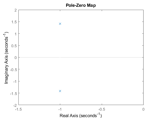
Pole analysis is a classic method of assessing the stability of a system. It involves looking at the locations of the poles in the pole-zero map, as shown in the figure. The poles of a system are found from its model, e.g., the transfer function model. If one of the poles is in the right-hand plane, then the system is unstable and you need to use feedback to stabilize it. Otherwise, your system is stable (or marginally stable) but you will still need feedback in order to get the desired response from the system, such as the motor position control.
Bounded Input Bounded Output (BIBO) is probably the most intuitive type of stability analysis. As an experimental method, it assesses the stability of a system based on the response when applying different bounded inputs. If a step input is applied to the system and its response keeps increasing, then the system is unstable.
The advantage of BIBO is that no model is needed. The drawback: it often cannot be used in hardware applications which, if get unstable, could be dangerous. Further, obtaining a clear stability definition from BIBO can be tricky. Pole analysis gives you a very clear assessment of the system stability but it requires an accurate model of the system, otherwise, the analysis will not be accurate.
Second-order Systems
There is a wide range of systems that are second-order, e.g., double spring-mass damper, pendulum. The properties of second-order systems are often used in time-domain control design. We introduce the concepts in the QUBE-Servo’s Proportional and the PD Control labs. Using QUBE-Servo 2 is an ideal way of learning about natural frequency, damping ratio, and how they relate to the servo’s speed response, i.e., peak time and overshoot.
Routh-Hurwitz Stability
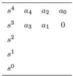
Routh-Hurwitz is another model-based stability analysis method. The major benefit of the Routh-Hurwitz Criterion is its inherent capability to determine the range for which unknown system parameters result in stable closed-loop system response. To do that, a Routh table is created based on the coefficients of the transfer function’s denominator. The table is used to find out how many poles are in the left-half plane, on the imaginary axis, or in the right-half plane.
In this lab, Routh-Hurwitz is applied to QUBE-Servo 2 to find the range of the control gain for which the system is stable. The assessment is first carried out theoretically and then tested on the actual system.
Nyquist Stability
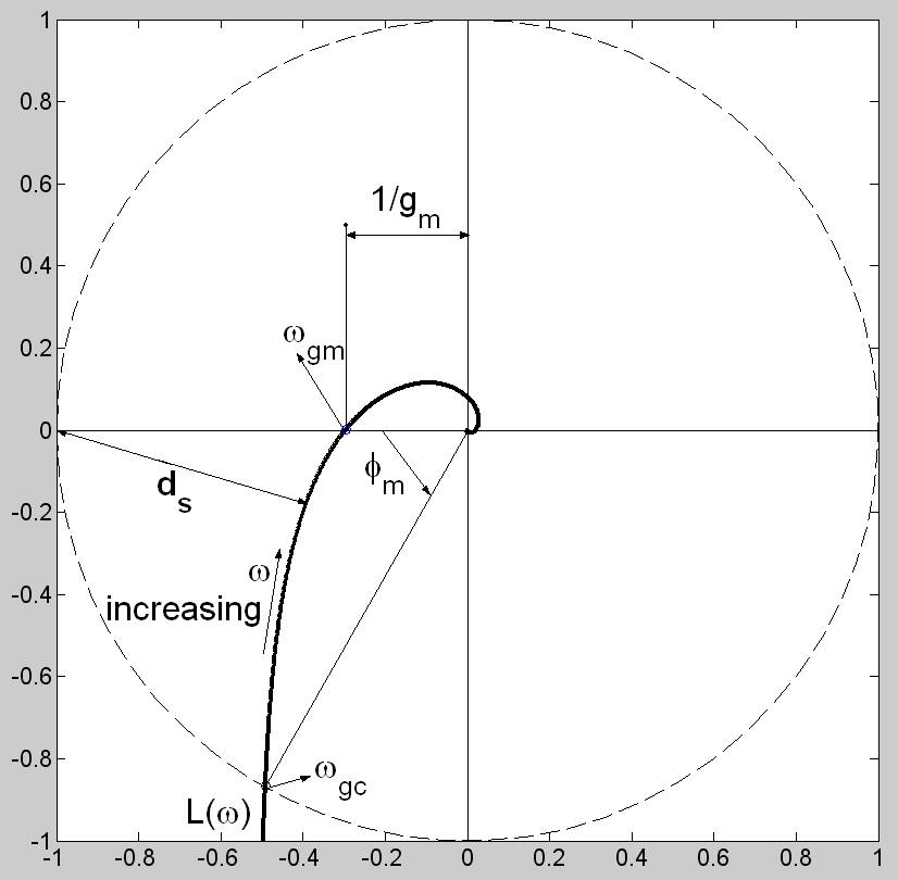
You can use the Nyquist diagram of a system to find the gain and phase margins of a system, which are key indicators of the system’s stability. The gain margin indicates how much open-loop gain is required before the system would go unstable. The phase margin indicates how much phase shift is needed in order to make the system go unstable. The phase margin also relates to a delay margin that indicates how many sample delays a system needs before going unstable.
In this lab, students get the opportunity to find the gain and delay margins of the QUBE-Servo 2 system experimentally, by adjusting the gain in the forward loop path and adding sampling delays. This is then compared with the stability margins found in the Nyquist analysis.
Why perform control design?
Controllers are used for stabilizing unstable systems and make them behave in a certain way. For example, Proportional-Derivative (PD) control is commonly implemented to change the position of a DC motor or a robot manipulator joint.
Overview of QUBE-Servo 2 Control Design labs
The control design labs supplied with QUBE-Servo 2 are listed below:
| Lab | Description |
| Proportional Control | Implement a proportional control to perform DC motor position and speed setpoint tracking. Assess the steady-state error in each case. |
| PD control | Design a PD control to perform motor position tracking based on step response design requirements. |
| Lead Compensator | Design a lead compensator to perform motor position control based on the frequency and time-domain requirements. |
| Steady-State Error | Assess the steady-state error using different controllers and reference signals. Identify the “System Type” based on your analysis. |
| Load Disturbance | Design a controller that can compensate for disturbances acting on the inertial disk of the servo. |
| Robustness | Design a PD control based on the Minimum Sensitivity method that is more robust against parameter variations. |
| Optimal Control | Design and test a Linear-Quadratic Regulator (LQR) optimal control to control the position of the DC motor. |
Proportional Control
Proportional-Integral-Derivative (PID) is the most widely used type of control. Programmable Logic Circuits (PLCs) typically use PID control for automation applications in a wide range of industries. Proportional control typically supplies the majority of the control effort and is a great way to start learning about the PID family of control.
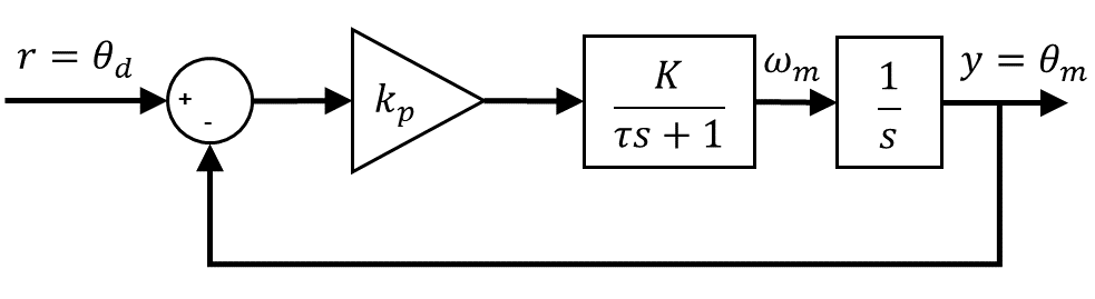
In the QUBE-Servo 2 lab, students design a proportional compensator to control the position and speed of the servo DC motor in order to meet certain performance requirements. While the control design for a proportional control is the simplest, the lab demonstrates that using this method alone has some drawbacks.
PD Control
Proportional-Derivative (PD) control is often used in fast-moving motion control systems such as servos, pick and place robots, and so on. It solves some of the drawbacks of using only the proportional control.
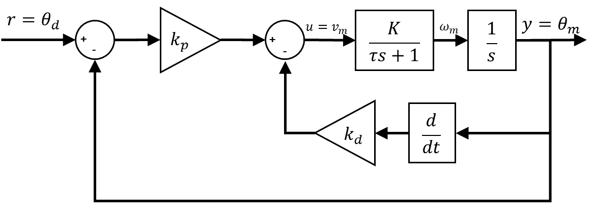
Similarly to the Proportional Control lab, the PD gains are designed to meet certain performance requirements, i.e. peak time and overshoot, which were introduced in the Second Order Systems lab.
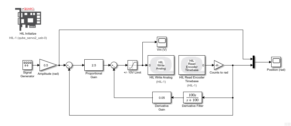
Running PD control on the QUBE-Servo 2 system gives students an intuitive understanding of how the proportional and derivative terms affect the response. It also demonstrates how an ideal PD control can be problematic when implemented on hardware. Taking the direct derivative of the measured motor position response can lead to high-frequency noise, which is then fed back to the DC motor. In order to avoid this and ensure the control signal is smooth, filtering must be included (note: filtering is discussed in the Filtering lab). Here is the actual PD control that is implemented in Simulink with the Quanser QUARC software:
Lead Compensator
After PID, lead-lag compensation is probably the second most popular type of control used. A lead compensator is essentially a PD control with filtering, while lag compensation is a variation of a PI control.
In the QUBE-Servo 2 lab, a lead compensator is designed to control the speed of the DC motor. The design of a lead compensator is performed in the frequency domain and is very different from the time-domain-based design that was performed in the Proportional Control and PD Control labs. However, similar to these labs, the lead compensator is designed to meet certain specifications. The block diagram of the servo speed control using a lead compensator is shown here:
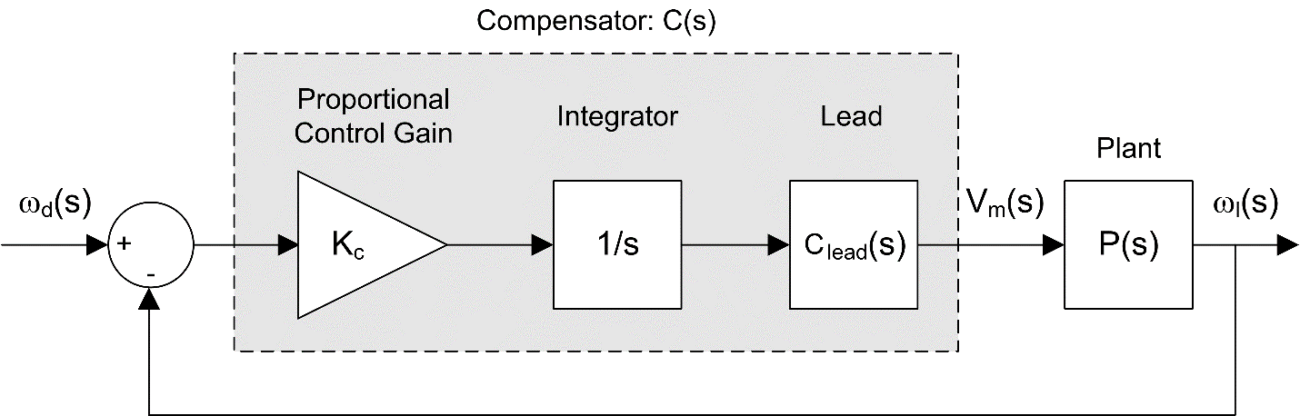
Lead compensators, because they already included filtering, don’t need special modifications to be implemented, as in case of PD control. But lead compensation alone can result in a large steady-state error, which is why an integral is used in the controller, as illustrated in the block diagram above.
Steady-state error
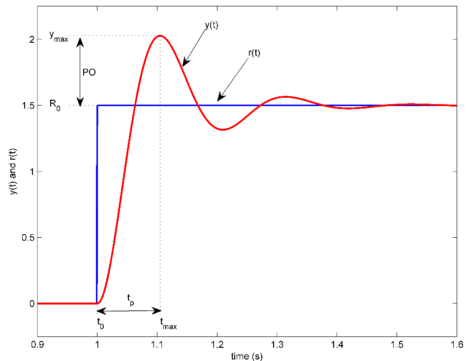
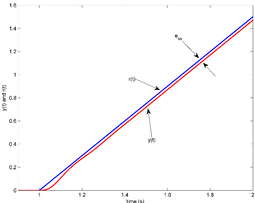
Steady-state error is the error between the reference signal and the measured signal, as depicted in the response below. It an important property in closed-loop systems, especially for high-precision applications like satellite positioning.
In this lab, the steady-state error of QUBE-Servo 2 when tracking step and ramp reference position commands is analyzed. Students compare PD and PID control both analytically and experimentally by running the controllers on the QUBE-Servo 2. That way, they learn first-hand how PD and PID affect the response of the servo. Further, using actual hardware highlights some sources of steady-state error that are not captured in transfer function analysis.
Load Disturbance
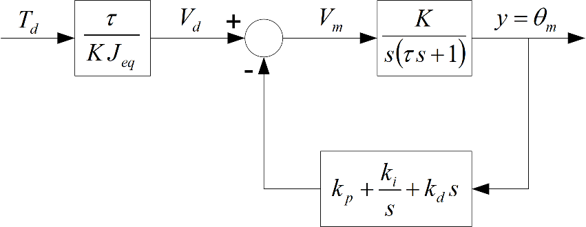
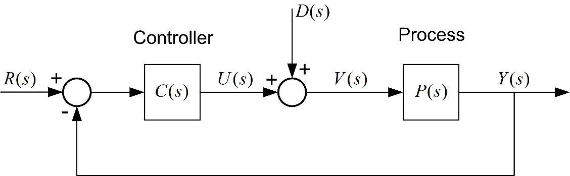
Disturbance rejection is the analysis of how a system responds to a disturbance, and how to compensate for it. For instance, a large gust of wind can cause an offset in the positioning of a satellite, which requires a controller to compensate for the disturbance.
In this case, the position response of the QUBE-Servo 2 system when a voltage disturbance is applied is examined using both PD and PID controllers. The analysis is first conducted by looking at the closed-loop system transfer functions, as shown in the block diagram below. Students then test how that correlates to the actual system using Simulink and the Quanser QUARC software.
Robustness
While the Load Disturbance lab involved looking at the system’s steady-state response due to a disturbance, the Robustness lab involves designing a controller based on how well it can handle process variations, known as Minimum Sensitivity Design (MSD). This is different from the tracking performance approach to control design that is based on time-domain specifications, such as rise time and overshoot, which is denoted as Speed Lab Design (SLD). Designing for minimum sensitivity also involves taking into account sampling and filtering effects, which impact the overall robustness of the system.
Students get to test how well the QUBE-Servo 2 system can withstand process variations and sample delays using the two types of control systems – the robust MSD controller and speed performance-based SLD control.
Optimal Control
In optimal control, a controller is designed based on certain user-defined parameters while trying to minimize the control effort. This is highly advantageous in systems where power conservation is at a premium, such as drones, or unmanned ground vehicles.
In addition to optimal control, this lab also introduces state feedback. So far, in all the previous labs, the control design was performed using transfer functions, known as the Classic Control design. State feedback is a Modern Control technique that uses the state-space representation of the system to design a controller. State feedback is typically used to control more complex, Multi-Input Multi-Output (MIMO) systems, but using it on a Single-Input Single-Output (SISO) servo is a great way to introduce students to the power of the method.
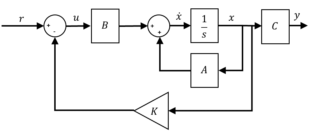
The general state-feedback control scheme is illustrated in the block diagram below. In this lab, state feedback is used to control the position of the QUBE-Servo 2. The state-feedback control gain, K, is found using the optimal control method known as a Linear Quadratic Regulator (LQR). LQR basically tries to minimize a cost function using the state-feedback control and, in doing so, generates a corresponding control gain K.
Using the QUBE-Servo 2 DC motor to learn about state-feedback and optimal control makes it much more intuitive for students. At the same time, it exposes them to more advanced, modern control techniques using a familiar application such as servo position control.
Stay tuned for the next blog post in which I will describe the discrete control labs in more detail.