

The QUBE-Servo 2 is supplied with two modules: the inertia disc and the pendulum. In my previous blog posts, I went through the various DC motor-based labs that use the disc module. Here I discuss the labs supplied with the QUBE-Servo 2 Pendulum system.
Why the pendulum?
The rotary pendulum system has been used in control labs for decades. The teaching benefits of pendulum are tremendous. The dynamics of a pendulum are similar to many real-world systems. The methods used to model a rotary pendulum system are the same ones used for robot manipulators and other multiple degree-of-freedom (DOF) systems. Using state-feedback and other control design approaches for the pendulum apply to a wide range of systems as well. I touched on this topic a while ago in my post Why is the pendulum so popular?
Overview of QUBE-Servo 2 Pendulum labs
The QUBE-Servo 2 includes seven pendulum-based labs that cater to the needs of typical control systems courses, from teaching introductory physics like finding the moment of inertia of a link to more advanced tasks like nonlinear control to swing-up the pendulum. They are summarized in the table below.
| Lab | Description |
| Moment of inertia | Find the moment of inertia of a pendulum analytically through first-principle physics and experimentally from the free-oscillation response. |
| Pendulum modelling | Make sure the system hardware matches the modelling conventions. This is an essential step to successful control system implementation. |
| State-space modelling | Represent the linearized model of the rotary pendulum in state-space and perform model validation. |
| Balance control | Implement a PD-based control to balance the pendulum in the inverted, upright position. |
| State-feedback Pole Placement control | Design a state-feedback control to balance the pendulum using the pole placement technique. |
| State-feedback LQR-based control | Design a state-feedback controller to balance the pendulum using the Linear Quadratic Regulator (LQR) optimal control method. |
| Swing-up control | Learn how to use an energy-based nonlinear control to swing-up the pendulum from its downward position to the inverted, upright position. |
Moment of Inertia
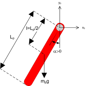
The moment of inertia is one of the main parameters in rotary systems. Having an accurate value is important in order to have a model that represents the actual system. In general, there are several ways to find the parameters of systems. In this case, we can find the inertia of the single-link pendulum analytically through the moment of inertia equation using the known mass and length of the link.
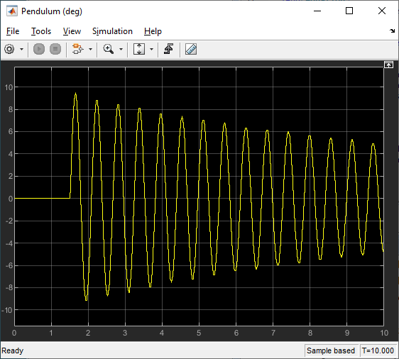
The other method is finding it experimentally by looking at the pendulum’s free-oscillation response and measuring its natural frequency.
Pendulum Modelling
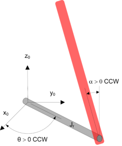
Making sure the hardware matches the model conventions is a crucial step in a control implementation procedure. Otherwise, the system can go unstable.
For example, if the pendulum on your rotary pendulum system goes positive when it rotates clockwise, but the model defines positive when rotating counter-clockwise, then your balance controller, which is based on the model of the system, will not be able to stabilize the system.
The Pendulum Modelling Lab requires that students actively test the system and ensure the sensor and actuator gains are set properly.
State-space Modelling
State-space representation was introduced as a new lab for the QUBE-Servo 2’s DC motor because it’s such an important technique to know in order to model more complex Multiple-Input Multiple-Output (MIMO) systems and use more advanced control methods.
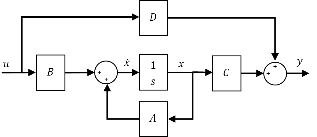
The rotary pendulum system is a single-input, multiple-output system: the DC motor is the input, and the rotary arm and pendulum angle positions and velocities are the outputs. As a result, rotary pendulum systems are typically modeled in state-space. In the lab, the state-space model is derived and then validated by comparing the open-loop response of the model with the actual system.
Balance Control
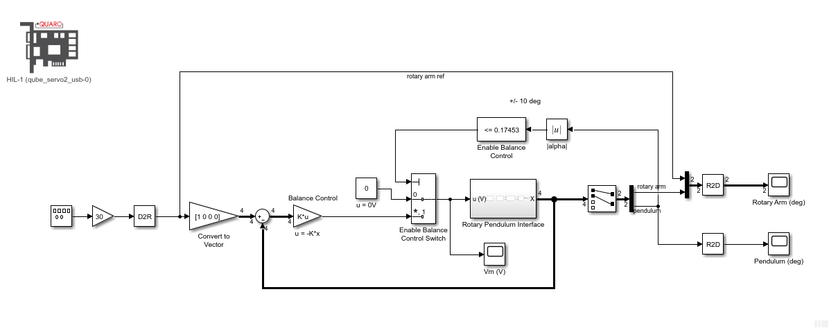
Balancing is a common control task found in many real-world systems, e.g., Segway or walking robots. While unconventional, this Pendulum Balance Lab uses a PD-based control to stabilize the pendulum in the upright, inverted position. This lab is meant as an introduction to the different components involved in such a task-based control application, including the control switching logic and measuring the inverted pendulum angle in order to balance it.
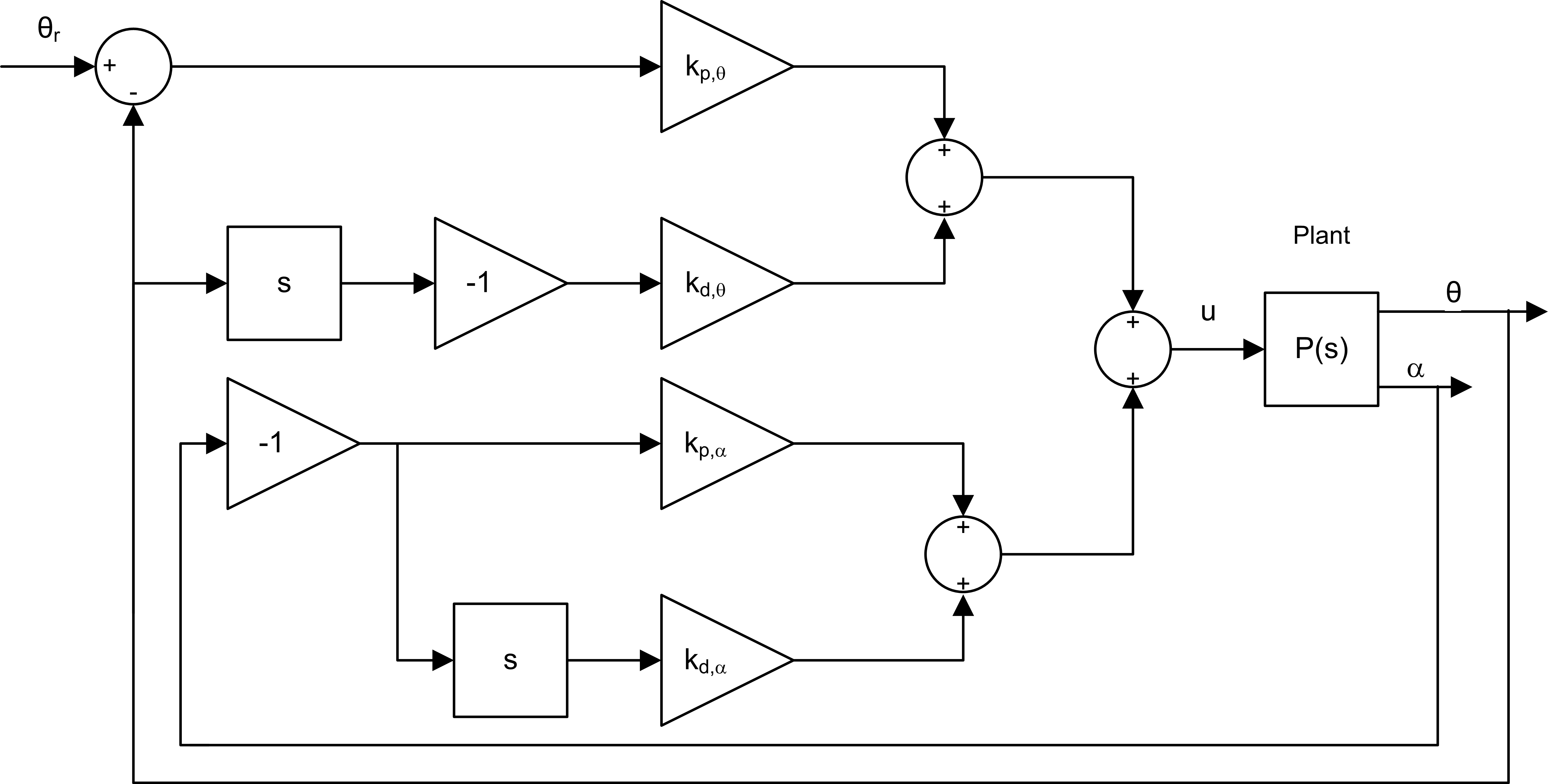
State-space modelling and control design are not needed for this lab, so students can learn how to balance a system using the more familiar PD control. However, the lab does highlight that state-space control techniques (or other advanced control methods) are needed to find control gains that will obtain a certain desired response.
State-feedback Pole Placement Control
State-feedback is the most common way of stabilizing an inverted pendulum, and pole placement is a standard technique used to find the control gain K for the closed-loop system shown below.
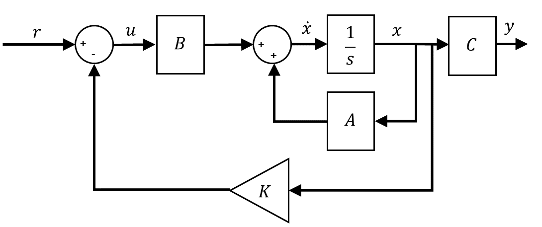
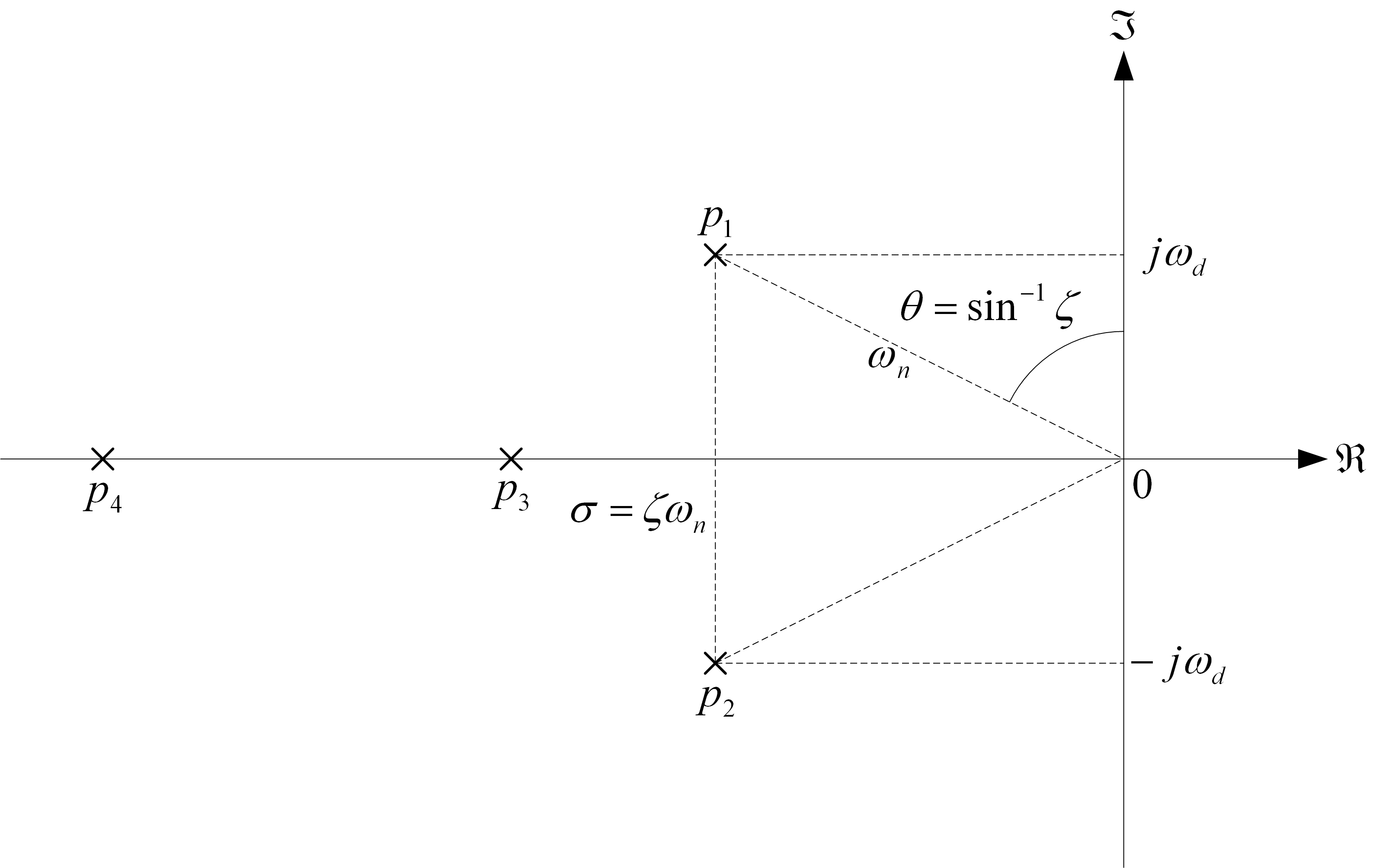
Pole placement finds a control gain that will drive the closed-loop poles of the system to the desired location. In this case, the desired pole locations are based on second-order time-domain requirements (i.e., percent overshoot and settling time), similar to what we introduced in the DC Motor PD Control Labs. From that, you can find the location of the two dominant poles, shown below as p1 and p2. The other two poles of the pendulum system are placed far along the real-axis in the left-hand plane. This technique is used in the control design of high-order systems.
The pole placement method is performed in the Matlab environment – both manually and using the Control System Toolbox function. Doing it manually exposes students to using companion matrices and gives them an idea of how the pole placement method helps find the control gain K. Then, they implement the controller on an actual system to see if the pendulum can balance and if it satisfies the controller requirements.
State-feedback LQR-based Control
Another very common technique to obtain the control gain K for state-feedback control is the Linear-Quadratic Regulator (LQR) optimization method. While the pole placement generates the control gain K needed to move the closed-loop poles to their desired locations, LQR minimizes a cost function that is based on the dynamics of the system and tuning matrices called weighting matrices. By placing different weights on the matrices, different control gains are generated.
Since LQR is an optimal control method, it finds a control gain that will obtain the best performance based on the weighting matrices selected while minimizing the control effort. This can be beneficial for systems with motor/actuator limitations (e.g., DC motor only allows +/- 5V), or for mobile systems that have limited battery power.
The method’s disadvantage is that finding the correct weighting matrices to satisfy the desired response is usually an iterative process. Pole placement is less of an iterative process as it finds the poles directly, based on the requirement. However, compared to LQR, pole placement tends to find control gain K that generates larger control signals.
Swing-up Control
Our Swing-up Control Lab introduces a simple nonlinear energy-based control. Similarly to a position or speed control where you have the desired position or speed setpoint, you can also have an energy setpoint. In this case, the setpoint is the energy of the pendulum when it is in the upright vertical position.

Based on the desired energy and the nonlinear dynamics of the pendulum, the swing-up algorithm finds the acceleration of the rotary arm that is needed to swing up the pendulum to the vertical position. The acceleration is converted into a motor voltage and then applied to the system. Once the pendulum swings up to a certain threshold about the vertical position, a state-feedback balance controller is engaged.
This is by no means a comprehensive nonlinear control design but it is a great way to introduce more advanced control techniques. You never know… it might motivate an undergraduate student to pursue graduate studies.
Final Notes
The techniques used to model, balance, and swing up an inverted pendulum have tremendous carry-over to other applications. State-space modelling is a mainstay to modeling more complex MIMO systems. State-feedback control is sometimes used in multi-DOF robot manipulators, quadrotor systems, aerospace devices, and so on. So, if you already have the QUBE-Servo 2 system in your lab, make sure to download the new set of labs.
By the way, the QUBE-Servo 2 is now also available virtually – check out QLabs Controls or QLabs Virtual QUBE-Servo 2. And don’t forget about our free mobile textbook app. It covers many of the topics that QUBE-Servo 2 labs focus on and is a great addition to your course and learning experience.